This is an example of analysis that can be done using the R-package mexhaz. This package allows to fit flexible hazard model in the framework of overall survival or net survival (i.e. excess hazard), with/wihout time-dependent effects for covariates, with/without non-linear effect and with/without random effect defined at the cluster level.
Start
The first step is to install the mexhaz package from the CRAN website. It needs to be done only the first time you’re using mexhaz, as the next time, mexhaz will be automatically pre-installed in your R session. To be able to use mexhaz in your R session, you need also to load the package by using the library() function.
Load the package
library(mexhaz)## Le chargement a nécessité le package : survivalsessionInfo()## R version 3.4.3 (2017-11-30)
## Platform: x86_64-w64-mingw32/x64 (64-bit)
## Running under: Windows 7 x64 (build 7601) Service Pack 1
##
## Matrix products: default
##
## locale:
## [1] LC_COLLATE=French_France.1252 LC_CTYPE=French_France.1252
## [3] LC_MONETARY=French_France.1252 LC_NUMERIC=C
## [5] LC_TIME=French_France.1252
##
## attached base packages:
## [1] methods stats graphics grDevices utils datasets base
##
## other attached packages:
## [1] mexhaz_1.3 survival_2.41-3
##
## loaded via a namespace (and not attached):
## [1] Rcpp_0.12.13 bookdown_0.6 lattice_0.20-35
## [4] digest_0.6.12 rprojroot_1.2 MASS_7.3-47
## [7] grid_3.4.3 backports_1.1.1 magrittr_1.5
## [10] evaluate_0.10.1 blogdown_0.5 stringi_1.1.5
## [13] Matrix_1.2-12 rmarkdown_1.6 splines_3.4.3
## [16] statmod_1.4.30 tools_3.4.3 stringr_1.2.0
## [19] numDeriv_2016.8-1 xfun_0.1 yaml_2.1.14
## [22] compiler_3.4.3 htmltools_0.3.6 knitr_1.18packageVersion("mexhaz")## [1] '1.3'oldPar <-par()Load the data
For this illustration, we will use the “simulated” data of colon cancer patients diagnosed in England between 2000 and 2002, and follow-up to the 31/12/2007.
sex: 1 for man, 2 for womansite: localisation of the cancer (Topography ICD-10)cancer: cancer sitediagmdy: date of diagnosisbirthmdy: date of birthdead: vital Status (0=Alive, 1=Death)finmdy: date of last know vital statusftime: survival Time in days (Follow-up maximum 7 years)stage: stage at diagnosisdep: deprivation group (5 categories)ageout: age at the last know vital status (integer)agediag: age at diagnosis (continuous)year: year at the last know vital statusgor: Government Office Region where the patient lived at the date of diagnosisid: identification numberagegrp: age at diagnosis in 5 categoriesrate: Population (Expected) mortality rate at the time of the last known vital status
We start to do some data management to work on complete data, and to create some useful variables
mydata <- read.delim(file="C:/Users/Aurélien/Dropbox/WorkStat/Teaching/Granada/Modelling/Practical/fakecolon_data.dat",
                     header = TRUE, sep = "\t", quote = "\"", dec = ".", fill = TRUE, comment.char = "")

temp <- mydata
temp <- temp[temp$dep!=9,]
temp <- temp[temp$sex==1,]

temp$timey <- temp$ftime/365.25

summary(temp)
## sex site cancer diagmdy
## Min. :1 C187 :6547 Colorectal:17867 10apr2002: 32
## 1st Qu.:1 C180 :3827 17apr2001: 32
## Median :1 C189 :2177 08dec2000: 29
## Mean :1 C182 :1788 23sep2002: 29
## 3rd Qu.:1 C184 :1188 03mar2002: 28
## Max. :1 C186 : 818 23may2002: 28
## (Other):1522 (Other) :17689
## birthmdy dead finmdy ftime
## 20jun1925: 8 Min. :0.0000 31dec2007: 3484 Min. : 1
## 03may1932: 7 1st Qu.:0.0000 23nov2007: 101 1st Qu.: 322
## 05mar1927: 7 Median :1.0000 16nov2007: 98 Median :1303
## 07aug1930: 7 Mean :0.6141 19dec2007: 93 Mean :1325
## 11jul1930: 7 3rd Qu.:1.0000 24nov2007: 92 3rd Qu.:2232
## 01jan1922: 6 Max. :1.0000 11dec2007: 91 Max. :2920
## (Other) :17825 (Other) :13908
## stage dep ageout agediag year
## A:1738 Min. :1.00 Min. :18.46 Min. :16.10 Min. :2000
## B:6959 1st Qu.:2.00 1st Qu.:68.14 1st Qu.:64.25 1st Qu.:2002
## C:6360 Median :3.00 Median :75.79 Median :72.14 Median :2005
## D:2810 Mean :2.96 Mean :74.35 Mean :70.73 Mean :2004
## 3rd Qu.:4.00 3rd Qu.:81.91 3rd Qu.:78.51 3rd Qu.:2007
## Max. :5.00 Max. :99.00 Max. :99.09 Max. :2007
##
## gor id agegrp rate
## M:17867 Min. : 1 Min. :15.00 Min. :0.000444
## 1st Qu.: 8266 1st Qu.:55.00 1st Qu.:0.020526
## Median :15885 Median :65.00 Median :0.045229
## Mean :16354 Mean :65.37 Mean :0.062192
## 3rd Qu.:23997 3rd Qu.:75.00 3rd Qu.:0.085530
## Max. :34731 Max. :85.00 Max. :0.559850
##
## timey
## Min. :0.002738
## 1st Qu.:0.881588
## Median :3.567420
## Mean :3.628704
## 3rd Qu.:6.110883
## Max. :7.994524
## temp$agegrp <- rep("[15;45[")
temp$agegrp <- ifelse(temp$agediag>=45 & temp$agediag<55, "[45;55[", temp$agegrp)
temp$agegrp <- ifelse(temp$agediag>=55 & temp$agediag<65, "[55;65[", temp$agegrp)
temp$agegrp <- ifelse(temp$agediag>=65 & temp$agediag<75, "[65;75[", temp$agegrp)
temp$agegrp <- ifelse(temp$agediag>=75 , "[75;++[", temp$agegrp)
temp$agediagtrunc <- trunc(temp$agediag)
table(temp$agediagtrunc, temp$agegrp)##
## [15;45[ [45;55[ [55;65[ [65;75[ [75;++[
## 16 1 0 0 0 0
## 18 1 0 0 0 0
## 19 1 0 0 0 0
## 20 3 0 0 0 0
## 21 5 0 0 0 0
## 22 5 0 0 0 0
## 23 1 0 0 0 0
## 24 1 0 0 0 0
## 25 2 0 0 0 0
## 26 1 0 0 0 0
## 27 5 0 0 0 0
## 28 1 0 0 0 0
## 29 4 0 0 0 0
## 30 4 0 0 0 0
## 31 13 0 0 0 0
## 32 11 0 0 0 0
## 33 12 0 0 0 0
## 34 19 0 0 0 0
## 35 15 0 0 0 0
## 36 15 0 0 0 0
## 37 23 0 0 0 0
## 38 30 0 0 0 0
## 39 27 0 0 0 0
## 40 30 0 0 0 0
## 41 27 0 0 0 0
## 42 40 0 0 0 0
## 43 43 0 0 0 0
## 44 61 0 0 0 0
## 45 0 62 0 0 0
## 46 0 53 0 0 0
## 47 0 62 0 0 0
## 48 0 86 0 0 0
## 49 0 81 0 0 0
## 50 0 101 0 0 0
## 51 0 135 0 0 0
## 52 0 160 0 0 0
## 53 0 177 0 0 0
## 54 0 214 0 0 0
## 55 0 0 228 0 0
## 56 0 0 254 0 0
## 57 0 0 247 0 0
## 58 0 0 300 0 0
## 59 0 0 293 0 0
## 60 0 0 321 0 0
## 61 0 0 358 0 0
## 62 0 0 370 0 0
## 63 0 0 449 0 0
## 64 0 0 468 0 0
## 65 0 0 0 501 0
## 66 0 0 0 530 0
## 67 0 0 0 532 0
## 68 0 0 0 516 0
## 69 0 0 0 615 0
## 70 0 0 0 663 0
## 71 0 0 0 672 0
## 72 0 0 0 664 0
## 73 0 0 0 712 0
## 74 0 0 0 677 0
## 75 0 0 0 0 730
## 76 0 0 0 0 765
## 77 0 0 0 0 692
## 78 0 0 0 0 643
## 79 0 0 0 0 646
## 80 0 0 0 0 630
## 81 0 0 0 0 548
## 82 0 0 0 0 422
## 83 0 0 0 0 316
## 84 0 0 0 0 315
## 85 0 0 0 0 300
## 86 0 0 0 0 234
## 87 0 0 0 0 206
## 88 0 0 0 0 166
## 89 0 0 0 0 114
## 90 0 0 0 0 71
## 91 0 0 0 0 59
## 92 0 0 0 0 35
## 93 0 0 0 0 28
## 94 0 0 0 0 23
## 95 0 0 0 0 11
## 96 0 0 0 0 6
## 98 0 0 0 0 4
## 99 0 0 0 0 1quantile(temp$agediag, na.rm=T, probs = seq(0,1,0.1))## 0% 10% 20% 30% 40% 50% 60% 70%
## 16.10404 56.14565 62.11964 66.08515 69.41656 72.13689 74.72690 77.17509
## 80% 90% 100%
## 79.86311 83.32211 99.08556temp$Iagegrp1545 <- ifelse(temp$agegrp=="[15;45[",1,0)
temp$Iagegrp4555 <- ifelse(temp$agegrp=="[45;55[",1,0)
temp$Iagegrp5565 <- ifelse(temp$agegrp=="[55;65[",1,0)
temp$Iagegrp6575 <- ifelse(temp$agegrp=="[65;75[",1,0)
temp$Iagegrp75pp <- ifelse(temp$agegrp=="[75;++[",1,0)
# table(temp$Iagegrp1545, temp$agegrp)
# table(temp$Iagegrp4555, temp$agegrp)
# table(temp$Iagegrp5565, temp$agegrp)
# table(temp$Iagegrp6575, temp$agegrp)
# table(temp$Iagegrp75pp, temp$agegrp)
temp$agediagc=temp$agediag-70
temp$agediagc2 <- temp$agediagc^2
temp$agediagc2plus <- (temp$agediagc-0)^2*(temp$agediagc>0)
temp$agediagc3 <- temp$agediagc^3
temp$agediagc3plus <- (temp$agediagc-0)^3*(temp$agediagc>0)
temp$IstageA <- ifelse(temp$stage=="A",1,0) # table(temp$IstageA,temp$Dukesstage)
temp$IstageB <- ifelse(temp$stage=="B",1,0) # table(temp$IstageB,temp$Dukesstage)
temp$IstageC <- ifelse(temp$stage=="C",1,0) # table(temp$IstageC,temp$Dukesstage)
temp$IstageD <- ifelse(temp$stage=="D",1,0) # table(temp$IstageD,temp$Dukesstage)
temp$Idep1 <- ifelse(temp$dep==1,1,0) # table(temp$Idep1, temp$dep)
temp$Idep2 <- ifelse(temp$dep==2,1,0) # table(temp$Idep2, temp$dep)
temp$Idep3 <- ifelse(temp$dep==3,1,0) # table(temp$Idep3, temp$dep)
temp$Idep4 <- ifelse(temp$dep==4,1,0) # table(temp$Idep4, temp$dep)
temp$Idep5 <- ifelse(temp$dep==5,1,0) # table(temp$Idep5, temp$dep)
summary(temp$agediag)## Min. 1st Qu. Median Mean 3rd Qu. Max.
## 16.10 64.25 72.14 70.73 78.51 99.09summary(temp$timey)## Min. 1st Qu. Median Mean 3rd Qu. Max.
## 0.002738 0.881588 3.567420 3.628704 6.110883 7.994524table(temp$sex)##
## 1
## 17867table(temp$dep, temp$stage)##
## A B C D
## 1 341 1361 1249 548
## 2 383 1455 1375 580
## 3 344 1476 1308 554
## 4 372 1426 1329 575
## 5 298 1241 1099 553First Model: Age analysed as categorical variable
We fit a model M1bs assuming a cubic B-spline function for the (log of the) baseline excess hazard (using arguments base="exp.bs" and degree=3), with one knot located at 1 year (using argument knots to specify the location of the knot(s)). The model M1bs assumes linear and proportional (i.e. constant over time) effects of the covariables dep, stage and agegrp, the latter variable corresponding to the age at diagnosis categorised in age-group. We use the age-group [65-75[ as the reference for the variable agegrp. The results given by the mexhaz function are detailed below. The excess mortality hazard fitted is of the form \[ \lambda_E(t; x) = \lambda_0(t)\exp \big(\sum_{i=2}^4 \alpha_i stage_i + \sum_{i=2}^5 \beta_i dep_i + \sum_{i=1, i\ne 4}^5 \gamma_i agecat_i \big)\]. We also fit a model M1ns assuming a cubic restricted spline function for the (log of the) baseline excess hazard (using arguments base="exp.ns" and degree=3), with three interior knots located at 1, 3 and 5 years (using argument knots to specify the location of the knot(s)). The excess mortality hazard fitted is of the form \[ \lambda_E(t; x) = \lambda^{ns}_0(t)\exp \big(\sum_{i=2}^4 \alpha_i stage_i + \sum_{i=2}^5 \beta_i dep_i + \sum_{i=1, i\ne 4}^5 \gamma_i agecat_i \big)\].
Estimation
# M1overal <- mexhaz(Surv(timey, dead)~Idep2+Idep3+Idep4+Idep5+IstageB+IstageC+IstageD+Iagegrp1545+Iagegrp4555+Iagegrp5565+Iagegrp75pp,
#                 data=temp, base="exp.bs", degree=3, knots=c(1), verbose = 0)
#
# initial <- round(M1overal$coeff,2)

M1bs <- mexhaz(Surv(timey, dead)~Idep2+Idep3+Idep4+Idep5+IstageB+IstageC+IstageD+Iagegrp1545+Iagegrp4555+Iagegrp5565+Iagegrp75pp,
             data=temp, base="exp.bs", degree=3, knots=c(1), verbose = 500, expected="rate") # , init=initial)
## Eval LogLik Time
## 0 -25865.62 0.15
## Param
## [1] -1 -1 -1 -1 -1 0 0 0 0 0 0 0 0 0 0 0
##
## iteration = 0
## Step:
## [1] 0 0 0 0 0 0 0 0 0 0 0 0 0 0 0 0
## Parameter:
## [1] -1 -1 -1 -1 -1 0 0 0 0 0 0 0 0 0 0 0
## Function Value
## [1] 25865.62
## Gradient:
## [1] 1250.65358 60.29418 712.41550 826.00875 448.79197
## [6] 390.35978 280.70016 149.20958 26.07932 2255.47749
## [11] -149.00131 -1707.73004 66.95293 144.76583 537.96909
## [16] -95.52193
##
## Eval LogLik Time
## 500 -21874.37 19
## Param
## [1] -2.1240 -1.8421 -0.7866 -3.7884 -3.2131 -0.0051 0.0664 0.1178
## [9] 0.2143 0.8243 1.8281 3.1658 -0.2450 -0.1038 -0.1264 0.3309
##
## iteration = 54
## Parameter:
## [1] -2.141865427 -1.860586763 -0.715698489 -3.963560050 -2.954318210
## [6] -0.006557109 0.065265093 0.116906733 0.212574231 0.845157214
## [11] 1.849196579 3.187384801 -0.240507554 -0.102819529 -0.126464263
## [16] 0.331999008
## Function Value
## [1] 21874.03
## Gradient:
## [1] -0.0091159006 -0.0067789757 -0.0005456968 0.0003432783 0.0003854315
## [6] -0.0014479156 -0.0002983143 -0.0003019522 -0.0062645995 -0.0011496013
## [11] -0.0045110863 -0.0031307722 -0.0003383320 0.0020154403 -0.0032850949
## [16] -0.0010295480
##
## Gradient relatif proche de zéro.
## L'itération courante est probablement la solution.
##
## Computation of the Hessian
##
## Data
## Name N.Obs.Tot N.Obs N.Events N.Clust
## temp 17867 17867 10972 1
##
## Details
## Iter Eval Base Nb.Leg Nb.Aghq Optim Method Code LogLik Total.Time
## 54 823 exp.bs 20 10 nlm --- 1 -21874.03 31.09summary(M1bs)## Call:
## mexhaz(formula = Surv(timey, dead) ~ Idep2 + Idep3 + Idep4 +
## Idep5 + IstageB + IstageC + IstageD + Iagegrp1545 + Iagegrp4555 +
## Iagegrp5565 + Iagegrp75pp, data = temp, expected = "rate",
## base = "exp.bs", degree = 3, knots = c(1), verbose = 500)
##
## Coefficients:
## Estimate StdErr t.value p.value
## Intercept -2.1418654 0.1130108 -18.9527 < 2.2e-16 ***
## BS3.1 -1.8605868 0.0631538 -29.4612 < 2.2e-16 ***
## BS3.2 -0.7156985 0.1269160 -5.6391 1.735e-08 ***
## BS3.3 -3.9635600 0.2549669 -15.5454 < 2.2e-16 ***
## BS3.4 -2.9543182 0.3248457 -9.0945 < 2.2e-16 ***
## Idep2 -0.0065571 0.0396616 -0.1653 0.8686889
## Idep3 0.0652651 0.0398074 1.6395 0.1011220
## Idep4 0.1169067 0.0394431 2.9639 0.0030413 **
## Idep5 0.2125742 0.0402629 5.2797 1.309e-07 ***
## IstageB 0.8451572 0.1076694 7.8496 4.410e-15 ***
## IstageC 1.8491966 0.1050998 17.5947 < 2.2e-16 ***
## IstageD 3.1873848 0.1056762 30.1618 < 2.2e-16 ***
## Iagegrp1545 -0.2405076 0.0777560 -3.0931 0.0019838 **
## Iagegrp4555 -0.1028195 0.0493388 -2.0839 0.0371790 *
## Iagegrp5565 -0.1264643 0.0354330 -3.5691 0.0003591 ***
## Iagegrp75pp 0.3319990 0.0300190 11.0596 < 2.2e-16 ***
## ---
## Signif. codes: 0 '***' 0.001 '**' 0.01 '*' 0.05 '.' 0.1 ' ' 1
##
## Hazard ratios (for proportional effect variables):
## Coef HR CI.lower CI.upper
## Idep2 -0.0066 0.9935 0.9192 1.0738
## Idep3 0.0653 1.0674 0.9873 1.1541
## Idep4 0.1169 1.1240 1.0404 1.2144
## Idep5 0.2126 1.2369 1.1430 1.3384
## IstageB 0.8452 2.3283 1.8854 2.8754
## IstageC 1.8492 6.3547 5.1716 7.8084
## IstageD 3.1874 24.2250 19.6927 29.8004
## Iagegrp1545 -0.2405 0.7862 0.6751 0.9157
## Iagegrp4555 -0.1028 0.9023 0.8191 0.9939
## Iagegrp5565 -0.1265 0.8812 0.8221 0.9446
## Iagegrp75pp 0.3320 1.3938 1.3141 1.4782
##
## log-likelihood: -21874.0252 (for 16 degree(s) of freedom)
##
## number of observations: 17867, number of events: 10972M1ns <- mexhaz(Surv(timey, dead)~Idep2+Idep3+Idep4+Idep5+IstageB+IstageC+IstageD+Iagegrp1545+Iagegrp4555+Iagegrp5565+Iagegrp75pp,
data=temp, base="exp.ns", knots=c(1,3,5), verbose = 500, expected="rate")## Eval LogLik Time
## 0 -27264.32 0.13
## Param
## [1] -1 -1 -1 -1 -1 0 0 0 0 0 0 0 0 0 0 0
##
## iteration = 0
## Step:
## [1] 0 0 0 0 0 0 0 0 0 0 0 0 0 0 0 0
## Parameter:
## [1] -1 -1 -1 -1 -1 0 0 0 0 0 0 0 0 0 0 0
## Function Value
## [1] 27264.32
## Gradient:
## [1] 5954.3076 1571.3816 206.2587 2198.5810 -1038.6589 1438.2777
## [7] 1251.4660 1077.5460 803.3186 4501.5014 1471.5020 -1489.3667
## [13] 200.4369 504.4960 1587.9870 1336.9654
##
## Eval LogLik Time
## 500 -22107.88 25.7
## Param
## [1] -2.7389 -0.6098 -2.4879 -3.7999 -0.9576 -0.0091 0.0615 0.1208
## [9] 0.2180 0.8776 1.9023 3.2589 -0.2135 -0.0873 -0.1187 0.3418
##
## Eval LogLik Time
## 1000 -22105.34 51.38
## Param
## [1] -2.6885 -0.6693 -2.3127 -4.0833 -1.5447 -0.0090 0.0617 0.1156
## [9] 0.2153 0.8374 1.8610 3.2164 -0.2439 -0.1036 -0.1283 0.3354
##
## iteration = 79
## Parameter:
## [1] -2.688662355 -0.669166739 -2.312592180 -4.083298423 -1.544859949
## [6] -0.009051424 0.061689040 0.115538601 0.215265243 0.837568881
## [11] 1.861086727 3.216506282 -0.243785120 -0.103578347 -0.128345652
## [16] 0.335432560
## Function Value
## [1] 22105.34
## Gradient:
## [1] -0.0065259112 0.0066356733 0.0032830958 -0.0014183784 0.0008406966
## [6] 0.0153704605 -0.0178843038 0.0021500455 -0.0064173946 -0.0018590072
## [11] -0.0041401827 0.0000000000 0.0010513759 0.0006330083 -0.0040090526
## [16] -0.0015861588
##
## Gradient relatif proche de zéro.
## L'itération courante est probablement la solution.
##
## Computation of the Hessian
##
## Data
## Name N.Obs.Tot N.Obs N.Events N.Clust
## temp 17867 17867 10972 1
##
## Details
## Iter Eval Base Nb.Leg Nb.Aghq Optim Method Code LogLik Total.Time
## 79 1164 exp.ns 20 10 nlm --- 1 -22105.34 61.17summary(M1ns)## Call:
## mexhaz(formula = Surv(timey, dead) ~ Idep2 + Idep3 + Idep4 +
## Idep5 + IstageB + IstageC + IstageD + Iagegrp1545 + Iagegrp4555 +
## Iagegrp5565 + Iagegrp75pp, data = temp, expected = "rate",
## base = "exp.ns", knots = c(1, 3, 5), verbose = 500)
##
## Coefficients:
## Estimate StdErr t.value p.value
## Intercept -2.6886624 0.1134329 -23.7027 < 2.2e-16 ***
## NS3.1 -0.6691667 0.0711504 -9.4050 < 2.2e-16 ***
## NS3.2 -2.3125922 0.1386946 -16.6740 < 2.2e-16 ***
## NS3.3 -4.0832984 0.1742215 -23.4374 < 2.2e-16 ***
## NS3.4 -1.5448599 0.2964812 -5.2107 1.903e-07 ***
## Idep2 -0.0090514 0.0398388 -0.2272 0.820270
## Idep3 0.0616890 0.0400005 1.5422 0.123041
## Idep4 0.1155386 0.0396297 2.9155 0.003556 **
## Idep5 0.2152652 0.0404320 5.3241 1.027e-07 ***
## IstageB 0.8375689 0.1097932 7.6286 2.492e-14 ***
## IstageC 1.8610867 0.1070805 17.3803 < 2.2e-16 ***
## IstageD 3.2165063 0.1076268 29.8857 < 2.2e-16 ***
## Iagegrp1545 -0.2437851 0.0778114 -3.1330 0.001733 **
## Iagegrp4555 -0.1035783 0.0494208 -2.0958 0.036110 *
## Iagegrp5565 -0.1283457 0.0355444 -3.6109 0.000306 ***
## Iagegrp75pp 0.3354326 0.0301965 11.1083 < 2.2e-16 ***
## ---
## Signif. codes: 0 '***' 0.001 '**' 0.01 '*' 0.05 '.' 0.1 ' ' 1
##
## Hazard ratios (for proportional effect variables):
## Coef HR CI.lower CI.upper
## Idep2 -0.0091 0.9910 0.9165 1.0715
## Idep3 0.0617 1.0636 0.9834 1.1504
## Idep4 0.1155 1.1225 1.0386 1.2131
## Idep5 0.2153 1.2402 1.1457 1.3425
## IstageB 0.8376 2.3107 1.8633 2.8656
## IstageC 1.8611 6.4307 5.2132 7.9326
## IstageD 3.2165 24.9408 20.1973 30.7985
## Iagegrp1545 -0.2438 0.7837 0.6728 0.9128
## Iagegrp4555 -0.1036 0.9016 0.8184 0.9933
## Iagegrp5565 -0.1283 0.8795 0.8204 0.9430
## Iagegrp75pp 0.3354 1.3985 1.3182 1.4838
##
## log-likelihood: -22105.3382 (for 16 degree(s) of freedom)
##
## number of observations: 17867, number of events: 10972Prediction
mytime <- seq(0.1,7,0.1)

predM1bsbase <- predict(M1bs, time.pts = mytime,
                        data.val = data.frame(Idep2=0, Idep3=0, Idep4=0, Idep5=0,
                                              IstageB=0, IstageC=0, IstageD=0,
                                              Iagegrp1545=0, Iagegrp4555=0, Iagegrp5565=0, Iagegrp75pp=0))

predM1bsagegrp4555 <- predict(M1bs, time.pts = mytime,
                              data.val = data.frame(Idep2=0, Idep3=0, Idep4=0, Idep5=0,
                                                    IstageB=0, IstageC=0, IstageD=0,
                                                    Iagegrp1545=0, Iagegrp4555=1, Iagegrp5565=0, Iagegrp75pp=0))

predM1bsagegrp75pp <- predict(M1bs, time.pts = mytime,
                              data.val = data.frame(Idep2=0, Idep3=0, Idep4=0, Idep5=0,
                                                    IstageB=0, IstageC=0, IstageD=0,
                                                    Iagegrp1545=0, Iagegrp4555=0, Iagegrp5565=0, Iagegrp75pp=1))

# Plot of the baseline excess mortality hazard and the corresponding net survival
par(mfrow=c(1,2), oma = c(0, 0, 2, 0))
plot(predM1bsbase, which="hazard", xlim=c(0,5),ylim=c(0,0.1),
     conf.int = T, main="Baseline excess \n mortality hazard", lwd=2)
axis(2,at=seq(0,0.2,by=0.02), tck=1,lty=8, lwd=0.1, labels=F, col="grey")

plot(predM1bsbase, which="surv", xlim=c(0,5), ylim=c(0.8,1),
     conf.int = T, main="Net survival \n (Reference group)", lwd=2)
axis(2,at=seq(0,1,by=0.05), tck=1,lty=8, lwd=0.1, labels=F, col="grey")
mtext("Model 1 (B-Spline)", outer = TRUE, cex = 1.5)
predM1nsbasens <- predict(M1ns, time.pts = mytime,
                          data.val = data.frame(Idep2=0, Idep3=0, Idep4=0, Idep5=0,
                                                IstageB=0, IstageC=0, IstageD=0,
                                                Iagegrp1545=0, Iagegrp4555=0, Iagegrp5565=0, Iagegrp75pp=0))

predM1nsagegrp4555ns <- predict(M1ns, time.pts = mytime,
                                data.val = data.frame(Idep2=0, Idep3=0, Idep4=0, Idep5=0,
                                                      IstageB=0, IstageC=0, IstageD=0,
                                                      Iagegrp1545=0, Iagegrp4555=1, Iagegrp5565=0, Iagegrp75pp=0))

predM1nsagegrp75ppns <- predict(M1ns, time.pts = mytime,
                                data.val = data.frame(Idep2=0, Idep3=0, Idep4=0, Idep5=0,
                                                      IstageB=0, IstageC=0, IstageD=0,
                                                      Iagegrp1545=0, Iagegrp4555=0, Iagegrp5565=0, Iagegrp75pp=1))

# Plot of the baseline excess mortality hazard and the corresponding net survival
par(mfrow=c(1,2), oma = c(0, 0, 2, 0))
plot(predM1nsbasens, which="hazard", xlim=c(0,5),ylim=c(0,0.1),
     conf.int = T, main="Baseline excess \n mortality hazard", lwd=2)
axis(2,at=seq(0,0.2,by=0.02), tck=1,lty=8, lwd=0.1, labels=F, col="grey")

plot(predM1nsbasens, which="surv", xlim=c(0,5), ylim=c(0.8,1),
     conf.int = T, main="Net survival \n (Reference group)", lwd=2)
axis(2,at=seq(0,1,by=0.05), tck=1,lty=8, lwd=0.1, labels=F, col="grey")
mtext("Model 1 (Restricted Cubic Spline)", outer = TRUE, cex = 1.5)
#re-initialise par() parameters
par(mfrow=c(1,1), oma=c(0,0,0,0))

# Plot of the excess mortality hazard for 3 age-groups
plot(predM1bsbase, which="hazard", xlim=c(0,5),ylim=c(0,0.1), conf.int = F, lwd=2,cex.axis=1.5, cex.lab=1.5)
points(predM1bsagegrp4555, which="hazard", col="red", conf.int = F, lwd=2)
points(predM1bsagegrp75pp, which="hazard", col="blue", conf.int = F, lwd=2)

axis(2,at=seq(0,0.2,by=0.02), tck=1,lty=8, lwd=0.1, labels=F, col="grey")
title("Excess mortality hazard for different age-groups", cex.main=1.5)
legend(0.5, 0.1, c("[65-75[, men, Stage A, Deprivation level 1 (the baseline)",
                   "[45-55[, men, Stage A, Deprivation level 1",
                   "[75-++[, men, Stage A, Deprivation level 1"),
       col=c("black", "red", "blue"), lty=c(1,2,4), lwd=3, cex=1.1)
# Plot of the net survival for 3 age-groups
plot(predM1bsbase, which="surv", xlim=c(0,5),ylim=c(0.78,1), conf.int = F, cex.axis=1.5, cex.lab=1.5, lwd=2)
points(predM1bsagegrp4555, which="surv", col="red", conf.int = F, lwd=2)
points(predM1bsagegrp75pp, which="surv", col="blue", conf.int = F, lwd=2)

axis(2,at=seq(0,1,by=0.05), tck=1,lty=8, lwd=0.1, labels=F, col="grey")
title("Net survival for different age-groups", cex.main=1.8)
legend(0.4,0.84,c("[65-75[, men, Stage A, Deprivation level 1 (the baseline)",
                  "[45-55[, men, Stage A, Deprivation level 1",
                  "[75-++[, men, Stage A, Deprivation level 1"),
       col=c("black", "red", "blue"), lty=c(1,2,4), lwd=3, cex=1.1)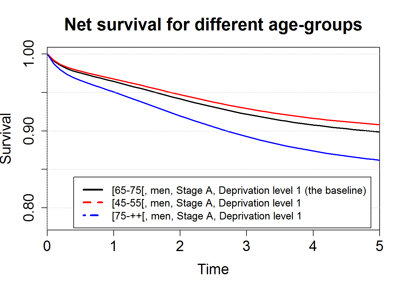
# Plot of the EHR for deprivation
HRdep <- data.frame(Estimates=exp(M1bs$coefficients[c("Idep2", "Idep3", "Idep4", "Idep5")]))
HRdep$LowBound <- exp(M1bs$coefficients[c("Idep2", "Idep3", "Idep4", "Idep5")]-qnorm(0.975)*M1bs$std.errors[c("Idep2", "Idep3", "Idep4", "Idep5")])
HRdep$UppBound <- exp(M1bs$coefficients[c("Idep2", "Idep3", "Idep4", "Idep5")]+qnorm(0.975)*M1bs$std.errors[c("Idep2", "Idep3", "Idep4", "Idep5")])

plot(x=seq(1,5), c(1,HRdep$Estimates), xlim=c(1,5), ylim=c(0.5,1.5),
     xlab="Deprivation quintiles", ylab="Excess Hazard Ratio", pch=18, lwd=3, cex.lab=1.5, cex.axis=1.5, cex=2)
axis(2, label=F, at=seq(0.5,2,by=0.1), tck=1,lty=8, lwd=0.1, col="grey")
axis(2, label=F, at=1, tck=1,lty=1, lwd=0.4)
for (i in seq(2,5)){arrows(i,HRdep$LowBound[i-1],i,HRdep$UppBound[i-1],code=3,length=0.2,angle=90,lwd=3)}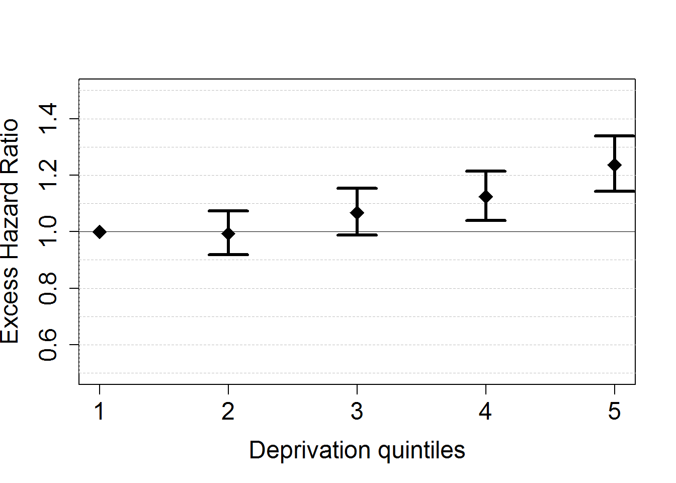
# Plot of the EHR for stage
HRstage <- data.frame(Estimates=exp(M1bs$coefficients[c("IstageB", "IstageC", "IstageD")]))
HRstage$LowBound <- exp(M1bs$coefficients[c("IstageB", "IstageC", "IstageD")]-qnorm(0.975)*M1bs$std.errors[c("IstageB", "IstageC", "IstageD")])
HRstage$UppBound <- exp(M1bs$coefficients[c("IstageB", "IstageC", "IstageD")]+qnorm(0.975)*M1bs$std.errors[c("IstageB", "IstageC", "IstageD")])

plot(seq(1,4), c(1, HRstage$Estimates), xlim=c(1,4), ylim=c(0.9,34),
     xlab="Stage", ylab="Excess Hazard Ratio (log scale)", pch=18, lwd=3, cex.lab=1.5, cex.axis=1.5, cex=2,
     log="y", xaxt="n")
axis(side=1, at=seq(1,4), labels=c("Stage A", "Stage B", "Stage C", "Stage D"), cex.axis=1.5)
axis(2, label=F, at=c(1,2,seq(4,34,by=2)), tck=1,lty=8, lwd=0.1, col="grey")
axis(2, label=F, at=1, tck=1,lty=1, lwd=0.2)
for (i in seq(1,3)){arrows(i+1,HRstage$LowBound[i],i+1,HRstage$UppBound[i],code=3,length=0.2,angle=90,lwd=3)}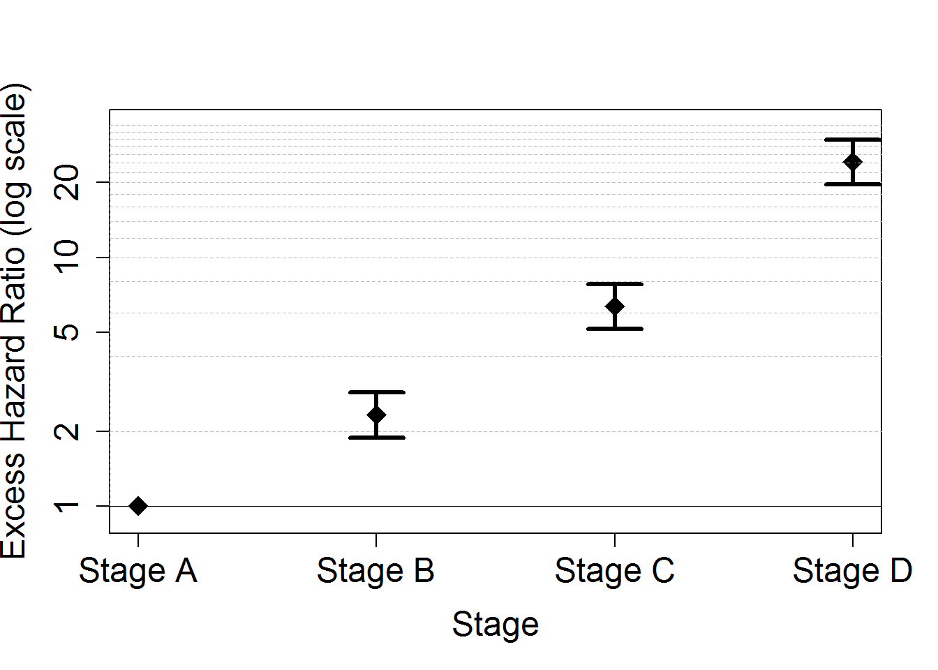
# Plot of the EHR for age-groups
HRageM1bs <- data.frame(Estimates=exp(M1bs$coefficients[c("Iagegrp1545", "Iagegrp4555", "Iagegrp5565", "Iagegrp75pp")]))
HRageM1bs$LowBound <- exp(M1bs$coefficients[c("Iagegrp1545", "Iagegrp4555", "Iagegrp5565", "Iagegrp75pp")]-qnorm(0.975)*M1bs$std.errors[c("Iagegrp1545", "Iagegrp4555", "Iagegrp5565", "Iagegrp75pp")])
HRageM1bs$UppBound <- exp(M1bs$coefficients[c("Iagegrp1545", "Iagegrp4555", "Iagegrp5565", "Iagegrp75pp")]+qnorm(0.975)*M1bs$std.errors[c("Iagegrp1545", "Iagegrp4555", "Iagegrp5565", "Iagegrp75pp")])

plot(0,0, type="n",xlab="Age at diagnosis", ylab="Excess Hazard Ratio ",
     xlim=c(15,99), ylim=c(0.4,2), lwd=3, cex.lab=1.5, cex.axis=1.5)
x.step<-c(15,45,55,65,75,99)
n.step<-length(x.step)
y.step<-c(HRageM1bs[,c("Estimates")][1:3], 1, HRageM1bs[,c("Estimates")][4])
for (j in 1:(n.step-1))
{lines(c(x.step[j],x.step[j+1]),c(y.step[j],y.step[j]), lwd=5 ,col=c("orange", "red", "purple", "black", "blue")[j])
}
axis(2, label=F, at=seq(0.5,1.9,by=0.1), tck=1,lty=8, lwd=0.1, col="grey")
axis(1, label=F, at=c(15,45,55,65,75,99), tck=1,lty=8, lwd=0.2, col="grey")
axis(2, label=F, at=1, tck=1,lty=1, lwd=0.2)
title("Excess hazard ratios for each age-group", cex.main=1.8)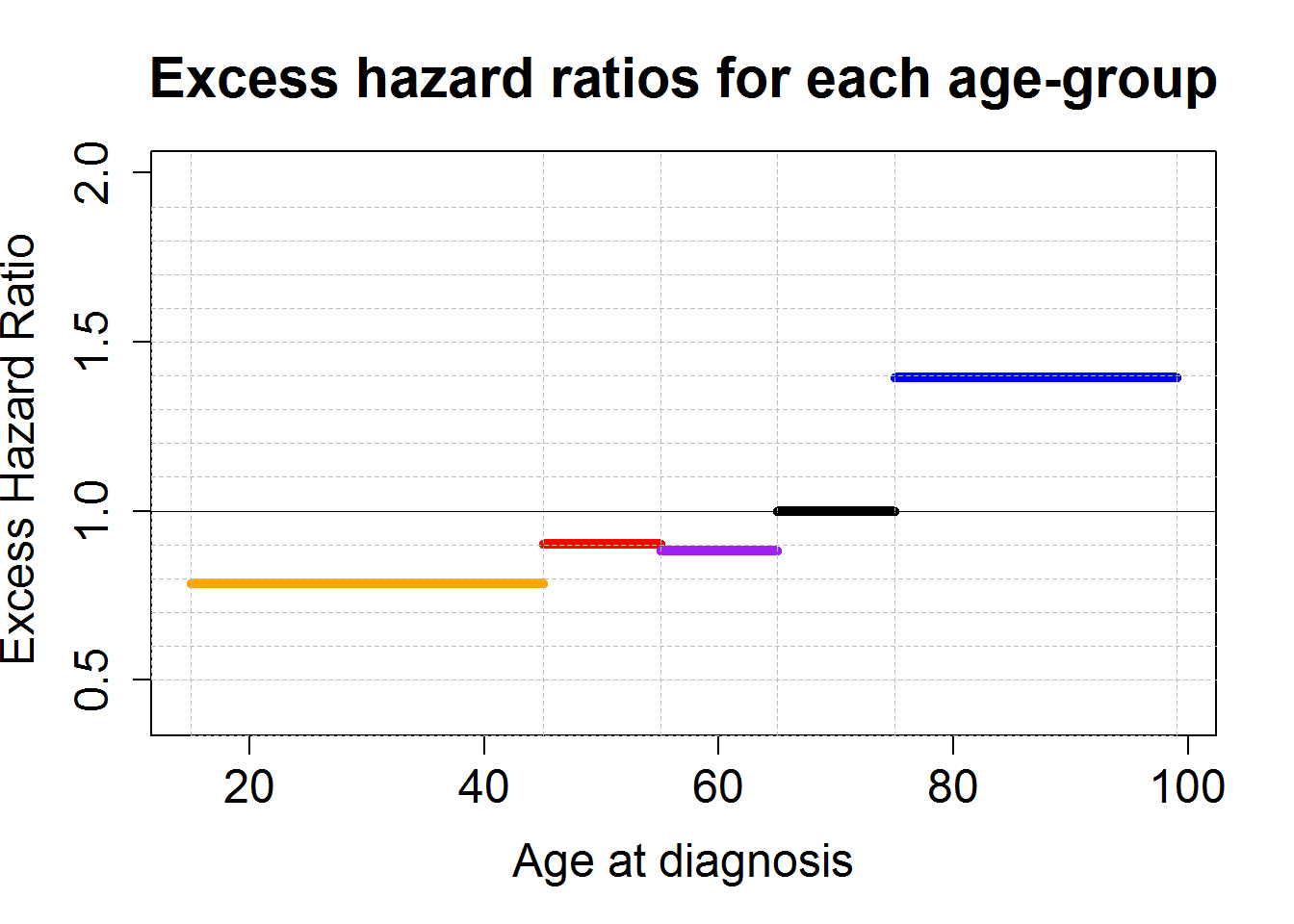
Second Model: Age analysed assuming a linear effect
We fit a model M2bs assuming a cubic B-spline function for the (log of the) baseline excess hazard (arguments base="exp.bs" and degree=3), with one knot located at 1 year (argument knots to specify the location of the knot(s)). The model M2bs assumes proportional (i.e. constant over time) effects of the covariables dep and stage, and a linear and proportional effect of continuous age. The excess mortality hazard fitted is of the form \[ \lambda_E(t; x) = \lambda_0(t)\exp \big(\sum_{i=2}^4 \alpha_i stage_i + \sum_{i=2}^5 \beta_i dep_i + \theta agec \big)\]. We also fit a model M2ns assuming a cubic restricted spline function for the (log of the) baseline excess hazard (using arguments base="exp.ns" and degree=3), with three interior knots located at 1, 3 and 5 years (using argument knots to specify the location of the knot(s)). The excess mortality hazard fitted is of the form \[ \lambda_E(t; x) = \lambda^{ns}_0(t)\exp \big(\sum_{i=2}^4 \alpha_i stage_i + \sum_{i=2}^5 \beta_i dep_i + \theta agec \big)\].
Estimation
M2bs <- mexhaz(Surv(timey, dead)~Idep2+Idep3+Idep4+Idep5+IstageB+IstageC+IstageD+agediagc,
               data=temp, base="exp.bs", degree=3, knots=c(1), verbose = 0,  expected="rate")
## iteration = 0
## Step:
## [1] 0 0 0 0 0 0 0 0 0 0 0 0 0
## Parameter:
## [1] -1 -1 -1 -1 -1 0 0 0 0 0 0 0 0
## Function Value
## [1] 25865.62
## Gradient:
## [1] 1250.65358 60.29418 712.41550 826.00875 448.79197
## [6] 390.35978 280.70016 149.20958 26.07932 2255.47749
## [11] -149.00131 -1707.73004 -11952.96934
##
## iteration = 136
## Parameter:
## [1] -2.051158417 -1.864230192 -0.716370111 -3.969809881 -2.927287512
## [6] -0.004077663 0.066438264 0.118533036 0.216144241 0.840944372
## [11] 1.840059212 3.183591187 0.017833676
## Function Value
## [1] 21880.73
## Gradient:
## [1] -7.981297e-04 4.039531e-04 -4.001777e-05 -3.583168e-04 -9.569418e-05
## [6] 4.438334e-04 2.386514e-03 -2.706656e-03 -6.511982e-04 -4.256435e-04
## [11] -2.669083e-04 -9.141824e-06 -7.919880e-03
##
## Gradient relatif proche de zéro.
## L'itération courante est probablement la solution.
##
## Computation of the Hessian
##
## Data
## Name N.Obs.Tot N.Obs N.Events N.Clust
## temp 17867 17867 10972 1
##
## Details
## Iter Eval Base Nb.Leg Nb.Aghq Optim Method Code LogLik Total.Time
## 136 1684 exp.bs 20 10 nlm --- 1 -21880.73 58.59summary(M2bs)## Call:
## mexhaz(formula = Surv(timey, dead) ~ Idep2 + Idep3 + Idep4 +
## Idep5 + IstageB + IstageC + IstageD + agediagc, data = temp,
## expected = "rate", base = "exp.bs", degree = 3, knots = c(1),
## verbose = 0)
##
## Coefficients:
## Estimate StdErr t.value p.value
## Intercept -2.0511584 0.1107754 -18.5164 < 2.2e-16 ***
## BS3.1 -1.8642302 0.0630470 -29.5689 < 2.2e-16 ***
## BS3.2 -0.7163701 0.1265172 -5.6622 1.517e-08 ***
## BS3.3 -3.9698099 0.2535376 -15.6577 < 2.2e-16 ***
## BS3.4 -2.9272875 0.3218373 -9.0956 < 2.2e-16 ***
## Idep2 -0.0040777 0.0396009 -0.1030 0.917989
## Idep3 0.0664383 0.0397208 1.6726 0.094417 .
## Idep4 0.1185330 0.0393795 3.0100 0.002616 **
## Idep5 0.2161442 0.0401820 5.3791 7.579e-08 ***
## IstageB 0.8409444 0.1069828 7.8606 4.041e-15 ***
## IstageC 1.8400592 0.1044068 17.6239 < 2.2e-16 ***
## IstageD 3.1835912 0.1049839 30.3246 < 2.2e-16 ***
## agediagc 0.0178337 0.0012109 14.7277 < 2.2e-16 ***
## ---
## Signif. codes: 0 '***' 0.001 '**' 0.01 '*' 0.05 '.' 0.1 ' ' 1
##
## Hazard ratios (for proportional effect variables):
## Coef HR CI.lower CI.upper
## Idep2 -0.0041 0.9959 0.9215 1.0763
## Idep3 0.0664 1.0687 0.9886 1.1552
## Idep4 0.1185 1.1258 1.0422 1.2162
## Idep5 0.2161 1.2413 1.1473 1.3430
## IstageB 0.8409 2.3186 1.8800 2.8595
## IstageC 1.8401 6.2969 5.1316 7.7269
## IstageD 3.1836 24.1333 19.6448 29.6473
## agediagc 0.0178 1.0180 1.0156 1.0204
##
## log-likelihood: -21880.7301 (for 13 degree(s) of freedom)
##
## number of observations: 17867, number of events: 10972M2ns <- mexhaz(Surv(timey, dead)~Idep2+Idep3+Idep4+Idep5+IstageB+IstageC+IstageD+agediagc,
data=temp, base="exp.ns", degree=3, knots=c(1, 3, 5), verbose = 0, expected="rate")## iteration = 0
## Step:
## [1] 0 0 0 0 0 0 0 0 0 0 0 0 0
## Parameter:
## [1] -1 -1 -1 -1 -1 0 0 0 0 0 0 0 0
## Function Value
## [1] 27264.32
## Gradient:
## [1] 5954.3076 1571.3816 206.2587 2198.5810 -1038.6589
## [6] 1438.2777 1251.4660 1077.5460 803.3186 4501.5014
## [11] 1471.5020 -1489.3667 -17972.3525
##
## iteration = 142
## Parameter:
## [1] -2.597302235 -0.669652784 -2.313216320 -4.069920815 -1.514917628
## [6] -0.006563437 0.062898402 0.117186398 0.218510063 0.833271022
## [11] 1.851551152 3.212173727 0.017925163
## Function Value
## [1] 22113.4
## Gradient:
## [1] -0.0006961360 -0.0001273293 0.0001431151 -0.0006248149 0.0003313983
## [6] -0.0001200533 -0.0002801244 0.0003165042 -0.0002728484 -0.0001055014
## [11] -0.0001611159 -0.0002763446 0.0108811946
##
## Gradient relatif proche de zéro.
## L'itération courante est probablement la solution.
##
## Computation of the Hessian
##
## Data
## Name N.Obs.Tot N.Obs N.Events N.Clust
## temp 17867 17867 10972 1
##
## Details
## Iter Eval Base Nb.Leg Nb.Aghq Optim Method Code LogLik Total.Time
## 142 1762 exp.ns 20 10 nlm --- 1 -22113.4 84.95summary(M2ns)## Call:
## mexhaz(formula = Surv(timey, dead) ~ Idep2 + Idep3 + Idep4 +
## Idep5 + IstageB + IstageC + IstageD + agediagc, data = temp,
## expected = "rate", base = "exp.ns", degree = 3, knots = c(1,
## 3, 5), verbose = 0)
##
## Coefficients:
## Estimate StdErr t.value p.value
## Intercept -2.5973022 0.1111495 -23.3676 < 2.2e-16 ***
## NS3.1 -0.6696528 0.0709573 -9.4374 < 2.2e-16 ***
## NS3.2 -2.3132163 0.1378527 -16.7804 < 2.2e-16 ***
## NS3.3 -4.0699208 0.1726073 -23.5791 < 2.2e-16 ***
## NS3.4 -1.5149176 0.2933062 -5.1650 2.431e-07 ***
## Idep2 -0.0065634 0.0397768 -0.1650 0.868940
## Idep3 0.0628984 0.0399127 1.5759 0.115066
## Idep4 0.1171864 0.0395657 2.9618 0.003062 **
## Idep5 0.2185101 0.0403506 5.4153 6.198e-08 ***
## IstageB 0.8332710 0.1090335 7.6423 2.241e-14 ***
## IstageC 1.8515512 0.1063132 17.4160 < 2.2e-16 ***
## IstageD 3.2121737 0.1068601 30.0596 < 2.2e-16 ***
## agediagc 0.0179252 0.0012172 14.7271 < 2.2e-16 ***
## ---
## Signif. codes: 0 '***' 0.001 '**' 0.01 '*' 0.05 '.' 0.1 ' ' 1
##
## Hazard ratios (for proportional effect variables):
## Coef HR CI.lower CI.upper
## Idep2 -0.0066 0.9935 0.9189 1.0740
## Idep3 0.0629 1.0649 0.9848 1.1516
## Idep4 0.1172 1.1243 1.0404 1.2150
## Idep5 0.2185 1.2442 1.1496 1.3466
## IstageB 0.8333 2.3008 1.8581 2.8491
## IstageC 1.8516 6.3697 5.1715 7.8455
## IstageD 3.2122 24.8330 20.1402 30.6193
## agediagc 0.0179 1.0181 1.0157 1.0205
##
## log-likelihood: -22113.3956 (for 13 degree(s) of freedom)
##
## number of observations: 17867, number of events: 10972Prediction
# plot linear effect of age (on log scale)
ageplot=(seq(15,90)-70)
binf.agediag=as.numeric(round(quantile(temp$agediag, na.rm=T, probs = c(0, 0.025, 0.25, 0.5, 0.75, 0.975, 1))[2],2))
bsup.agediag=as.numeric(round(quantile(temp$agediag, na.rm=T, probs = c(0, 0.025, 0.25, 0.5, 0.75, 0.975, 1))[6],2))


HRageM2bs <- exp(ageplot*M2bs$coefficients[c("agediagc")])
HRageM2ns <- exp(ageplot*M2ns$coefficients[c("agediagc")])
# Difference in EHR:
round(HRageM2bs-HRageM2ns,3)
## [1] 0.002 0.002 0.002 0.002 0.002 0.002 0.002 0.002 0.002 0.002
## [11] 0.002 0.002 0.002 0.002 0.002 0.002 0.002 0.002 0.002 0.002
## [21] 0.002 0.002 0.002 0.002 0.002 0.002 0.002 0.002 0.002 0.001
## [31] 0.001 0.001 0.001 0.001 0.001 0.001 0.001 0.001 0.001 0.001
## [41] 0.001 0.001 0.001 0.001 0.001 0.001 0.001 0.001 0.001 0.000
## [51] 0.000 0.000 0.000 0.000 0.000 0.000 0.000 0.000 0.000 0.000
## [61] -0.001 -0.001 -0.001 -0.001 -0.001 -0.001 -0.001 -0.001 -0.002 -0.002
## [71] -0.002 -0.002 -0.002 -0.002 -0.002 -0.003plot(ageplot+70, HRageM2bs, log="y", type="l",xlab="Age at diagnosis", ylab="Excess Hazard Ratio (log scale)",
xlim=c(binf.agediag,bsup.agediag), ylim=c(0.4,2), lwd=3, cex.lab=1.5, cex.axis=1.5)
lines(ageplot+70, HRageM2ns, lwd=3, lty=8, col="blue")
axis(2, label=F, at=seq(0.4,2,by=0.1), tck=1,lty=8, lwd=0.1, col="grey")
axis(2, label=F, at=1, tck=1,lty=1, lwd=0.5)
axis(1, label=F, at=70, tck=1,lty=8, lwd=0.1)
legend(50, 2, c("Cubic B-spline", "Restricted Cubic Spline"),
col=c("black", "blue"), lty=c(1,8), lwd=3, cex=1.3)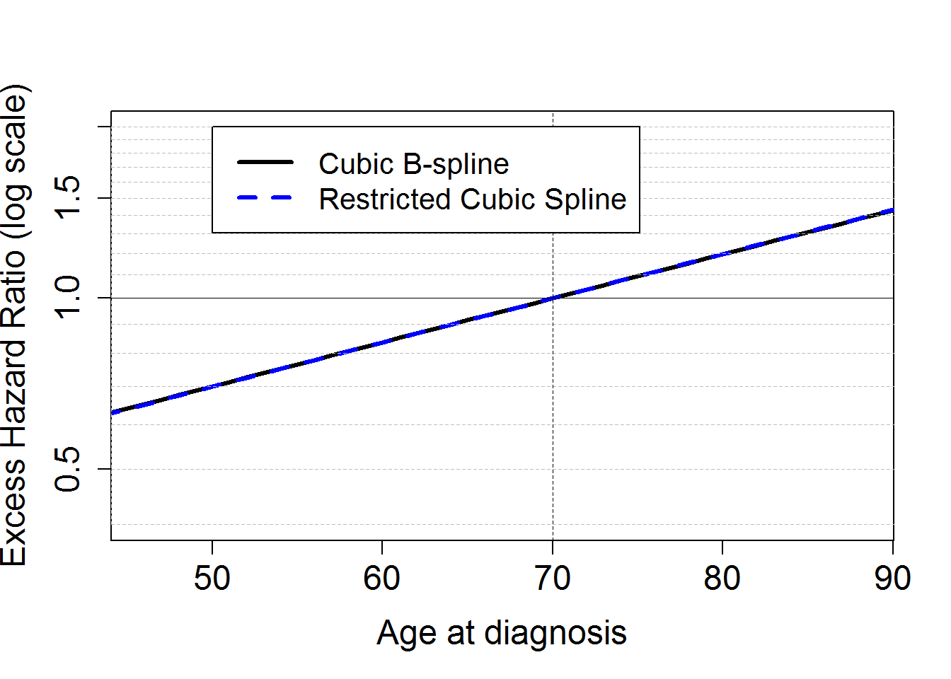
Third Model: Age analysed assuming a Non-linear effect
We fit a model M3bs assuming a cubic B-spline function for the (log of the) baseline excess hazard (arguments base="exp.bs" and degree=3), with one knot located at 1 year (argument knots to specify the location of the knot(s)). The model M3bs assumes proportional (i.e. constant over time) effects of the covariables dep and stage, and a non-linear and proportional effect of continuous age, by including 2 supplemental terms for age in the linear predictor (through the function \(f\). The excess mortality hazard fitted is of the form \[ \lambda_E(t; x) = \lambda_0(t)\exp \big(\sum_{i=2}^4 \alpha_i stage_i + \sum_{i=2}^5 \beta_i dep_i + \beta_a agec + f(agec) \big)\]. We also fit this model assuming a restrcited cubic spline for the (log of the) baseline excess hazard: M3ns.
Estimation
M3bs <- mexhaz(Surv(timey, dead)~Idep2+Idep3+Idep4+Idep5+IstageB+IstageC+IstageD+agediagc+ agediagc2+ agediagc2plus,
               data=temp, base="exp.bs", degree=3, knots=c(1), verbose = 0, expected="rate")
## iteration = 0
## Step:
## [1] 0 0 0 0 0 0 0 0 0 0 0 0 0 0 0
## Parameter:
## [1] -1 -1 -1 -1 -1 0 0 0 0 0 0 0 0 0 0
## Function Value
## [1] 25865.62
## Gradient:
## [1] 1250.65358 60.29418 712.41550 826.00875 448.79197
## [6] 390.35978 280.70016 149.20958 26.07932 2255.47749
## [11] -149.00131 -1707.73004 -11952.96934 124622.70458 -40400.48729
##
## iteration = 246
## Parameter:
## [1] -2.1201514937 -1.8587898394 -0.7004712283 -3.9634807198 -2.9253303092
## [6] -0.0094254953 0.0633182359 0.1129814002 0.2168466202 0.8221389681
## [11] 1.8261687421 3.1684398685 0.0153299290 0.0003192303 0.0009137206
## Function Value
## [1] 21840.06
## Gradient:
## [1] -8.584038e-03 -1.800484e-03 -3.232526e-04 -1.393210e-03 -1.490719e-04
## [6] -8.061761e-05 -9.102405e-04 -1.868466e-03 -6.879054e-04 -1.819099e-03
## [11] -3.072553e-03 -3.797555e-03 -4.119713e-01 4.919920e+02 2.181588e+01
##
## Le dernier pas global n'a pas pu localiser un point plus bas que x.
## Soit x est un mimimum local approximatif de la fonction,
## soit la fonction est par trop non linéaire pour cet algorithme,
## soit steptol est trop large.
##
## Computation of the Hessian
##
## Data
## Name N.Obs.Tot N.Obs N.Events N.Clust
## temp 17867 17867 10972 1
##
## Details
## Iter Eval Base Nb.Leg Nb.Aghq Optim Method Code LogLik Total.Time
## 246 3367 exp.bs 20 10 nlm --- 3 -21840.06 118.4summary(M3bs)## Call:
## mexhaz(formula = Surv(timey, dead) ~ Idep2 + Idep3 + Idep4 +
## Idep5 + IstageB + IstageC + IstageD + agediagc + agediagc2 +
## agediagc2plus, data = temp, expected = "rate", base = "exp.bs",
## degree = 3, knots = c(1), verbose = 0)
##
## Coefficients:
## Estimate StdErr t.value p.value
## Intercept -2.12015149 0.11060372 -19.1689 < 2.2e-16 ***
## BS3.1 -1.85878984 0.06284037 -29.5795 < 2.2e-16 ***
## BS3.2 -0.70047123 0.12676401 -5.5258 3.326e-08 ***
## BS3.3 -3.96348072 0.25464698 -15.5646 < 2.2e-16 ***
## BS3.4 -2.92533031 0.32447606 -9.0156 < 2.2e-16 ***
## Idep2 -0.00942550 0.03953574 -0.2384 0.811570
## Idep3 0.06331824 0.03963821 1.5974 0.110193
## Idep4 0.11298140 0.03932639 2.8729 0.004072 **
## Idep5 0.21684662 0.04014884 5.4011 6.709e-08 ***
## IstageB 0.82213897 0.10652390 7.7179 1.245e-14 ***
## IstageC 1.82616874 0.10393854 17.5697 < 2.2e-16 ***
## IstageD 3.16843987 0.10452984 30.3113 < 2.2e-16 ***
## agediagc 0.01532993 0.00271382 5.6488 1.640e-08 ***
## agediagc2 0.00031923 0.00010284 3.1042 0.001911 **
## agediagc2plus 0.00091372 0.00029399 3.1080 0.001887 **
## ---
## Signif. codes: 0 '***' 0.001 '**' 0.01 '*' 0.05 '.' 0.1 ' ' 1
##
## Hazard ratios (for proportional effect variables):
## Coef HR CI.lower CI.upper
## Idep2 -0.0094 0.9906 0.9168 1.0704
## Idep3 0.0633 1.0654 0.9857 1.1514
## Idep4 0.1130 1.1196 1.0365 1.2093
## Idep5 0.2168 1.2422 1.1481 1.3439
## IstageB 0.8221 2.2754 1.8466 2.8037
## IstageC 1.8262 6.2100 5.0654 7.6133
## IstageD 3.1684 23.7704 19.3666 29.1755
## agediagc 0.0153 1.0154 1.0101 1.0209
## agediagc2 0.0003 1.0003 1.0001 1.0005
## agediagc2plus 0.0009 1.0009 1.0003 1.0015
##
## log-likelihood: -21840.0601 (for 15 degree(s) of freedom)
##
## number of observations: 17867, number of events: 10972M3ns <- mexhaz(Surv(timey, dead)~Idep2+Idep3+Idep4+Idep5+IstageB+IstageC+IstageD+agediagc+ agediagc2+ agediagc2plus,
data=temp, base="exp.ns", degree=3, knots=c(1, 3, 5), verbose = 0, expected="rate")## iteration = 0
## Step:
## [1] 0 0 0 0 0 0 0 0 0 0 0 0 0 0 0
## Parameter:
## [1] -1 -1 -1 -1 -1 0 0 0 0 0 0 0 0 0 0
## Function Value
## [1] 27264.32
## Gradient:
## [1] 5954.3076 1571.3816 206.2587 2198.5810 -1038.6589
## [6] 1438.2777 1251.4660 1077.5460 803.3186 4501.5014
## [11] 1471.5020 -1489.3667 -17972.3525 668084.6915 132240.5401
##
## iteration = 251
## Parameter:
## [1] -2.6616493634 -0.6580455548 -2.3148111378 -4.0675392208 -1.5140238567
## [6] -0.0123443323 0.0596319177 0.1111507060 0.2186027457 0.8142118804
## [11] 1.8365222025 3.1957520438 0.0154776232 0.0003205005 0.0009259950
## Function Value
## [1] 22072.98
## Gradient:
## [1] -9.567696e-06 3.637979e-06 -4.714828e-06 -8.943930e-06 0.000000e+00
## [6] -7.275958e-06 -3.637979e-06 -3.637979e-06 -3.637979e-06 -3.637979e-06
## [11] -9.904533e-06 -4.553518e-06 4.365575e-05 -2.110028e-03 -4.001777e-04
##
## Gradient relatif proche de zéro.
## L'itération courante est probablement la solution.
##
## Computation of the Hessian
##
## Data
## Name N.Obs.Tot N.Obs N.Events N.Clust
## temp 17867 17867 10972 1
##
## Details
## Iter Eval Base Nb.Leg Nb.Aghq Optim Method Code LogLik Total.Time
## 251 3330 exp.ns 20 10 nlm --- 1 -22072.98 168.22summary(M3ns)## Call:
## mexhaz(formula = Surv(timey, dead) ~ Idep2 + Idep3 + Idep4 +
## Idep5 + IstageB + IstageC + IstageD + agediagc + agediagc2 +
## agediagc2plus, data = temp, expected = "rate", base = "exp.ns",
## degree = 3, knots = c(1, 3, 5), verbose = 0)
##
## Coefficients:
## Estimate StdErr t.value p.value
## Intercept -2.66164936 0.11090745 -23.9988 < 2.2e-16 ***
## NS3.1 -0.65804555 0.07110720 -9.2543 < 2.2e-16 ***
## NS3.2 -2.31481114 0.13874410 -16.6840 < 2.2e-16 ***
## NS3.3 -4.06753922 0.17378921 -23.4050 < 2.2e-16 ***
## NS3.4 -1.51402386 0.29561326 -5.1216 3.060e-07 ***
## Idep2 -0.01234433 0.03970346 -0.3109 0.755870
## Idep3 0.05963192 0.03981868 1.4976 0.134258
## Idep4 0.11115071 0.03950365 2.8137 0.004903 **
## Idep5 0.21860275 0.04030874 5.4232 5.930e-08 ***
## IstageB 0.81421188 0.10850816 7.5037 6.496e-14 ***
## IstageC 1.83652220 0.10578403 17.3611 < 2.2e-16 ***
## IstageD 3.19575204 0.10634660 30.0503 < 2.2e-16 ***
## agediagc 0.01547762 0.00273025 5.6689 1.459e-08 ***
## agediagc2 0.00032050 0.00010311 3.1085 0.001883 **
## agediagc2plus 0.00092600 0.00029742 3.1134 0.001852 **
## ---
## Signif. codes: 0 '***' 0.001 '**' 0.01 '*' 0.05 '.' 0.1 ' ' 1
##
## Hazard ratios (for proportional effect variables):
## Coef HR CI.lower CI.upper
## Idep2 -0.0123 0.9877 0.9138 1.0677
## Idep3 0.0596 1.0614 0.9818 1.1476
## Idep4 0.1112 1.1176 1.0343 1.2075
## Idep5 0.2186 1.2443 1.1498 1.3466
## IstageB 0.8142 2.2574 1.8249 2.7924
## IstageC 1.8365 6.2747 5.0997 7.7204
## IstageD 3.1958 24.4285 19.8321 30.0903
## agediagc 0.0155 1.0156 1.0102 1.0210
## agediagc2 0.0003 1.0003 1.0001 1.0005
## agediagc2plus 0.0009 1.0009 1.0003 1.0015
##
## log-likelihood: -22072.9753 (for 15 degree(s) of freedom)
##
## number of observations: 17867, number of events: 10972Prediction
HRageM3bs <- exp(ageplot*M3bs$coefficients[c("agediagc")] +
                   ageplot^2*M3bs$coefficients[c("agediagc2")] +
                   ageplot^2*M3bs$coefficients[c("agediagc2plus")]*(ageplot>0) )
HRageM3ns <- exp(ageplot*M3ns$coefficients[c("agediagc")] +
                   ageplot^2*M3ns$coefficients[c("agediagc2")] +
                   ageplot^2*M3ns$coefficients[c("agediagc2plus")]*(ageplot>0) )
# Difference in EHR:
round(HRageM3bs-HRageM3ns,3)
## [1] 0.005 0.005 0.005 0.005 0.004 0.004 0.004 0.004 0.004 0.004
## [11] 0.004 0.004 0.004 0.004 0.004 0.003 0.003 0.003 0.003 0.003
## [21] 0.003 0.003 0.003 0.003 0.003 0.003 0.003 0.003 0.003 0.002
## [31] 0.002 0.002 0.002 0.002 0.002 0.002 0.002 0.002 0.002 0.002
## [41] 0.002 0.002 0.001 0.001 0.001 0.001 0.001 0.001 0.001 0.001
## [51] 0.001 0.001 0.000 0.000 0.000 0.000 0.000 0.000 -0.001 -0.001
## [61] -0.001 -0.002 -0.002 -0.003 -0.003 -0.004 -0.004 -0.005 -0.006 -0.007
## [71] -0.009 -0.010 -0.012 -0.014 -0.016 -0.019varcovnlin <- M3bs$vcov[c("agediagc", "agediagc2plus", "agediagc2plus"), c("agediagc", "agediagc2plus", "agediagc2plus")]
# Confidence Intervals of Nlin effect
vary=NULL
for (i in c(ageplot)){vary <-c(vary, c(i, i^2, (i>0)*i^2) %*% varcovnlin %*% c(i, i^2, (i>0)*i^2))}
yLB <- HRageM3bs*exp(-qnorm(0.975)*sqrt(vary))
yUB <- HRageM3bs*exp(qnorm(0.975)*sqrt(vary))
plot(ageplot+70, HRageM3bs, log="y", type="n",xlab="Age at diagnosis", ylab="Excess Hazard Ratio (log scale)",
xlim=c(binf.agediag,bsup.agediag), ylim=c(0.4,2), lwd=3, cex.lab=1.5, cex.axis=1.5, col="blue")
polygon(c(ageplot+70,rev(ageplot+70)),c(yUB,rev(yLB)), col=grey(0.8), border=F)
lines(ageplot+70, HRageM3bs, lwd=3)
lines(ageplot+70, HRageM3ns, lwd=3, lty=8, col="blue")
axis(2, label=F, at=seq(0.4,2,by=0.1), tck=1,lty=8, lwd=0.1, col="grey")
axis(2, label=F, at=1, tck=1,lty=1, lwd=0.2)
axis(1, label=F, at=70, tck=1,lty=1, lwd=0.2)
legend(50, 2, c("Cubic B-spline", "Restricted Cubic Spline"),
col=c("black", "blue"), lty=c(1,8), lwd=3, cex=1.3)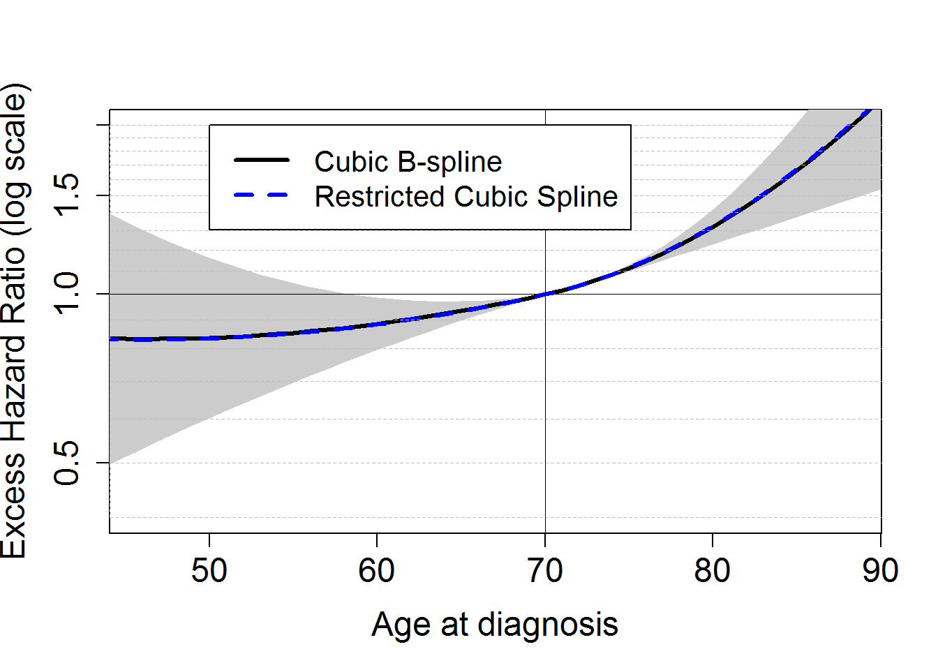
Comparison between first, second and third model
# Plot comparing the effect of age at diagnosis according to the different models: Categorical vs linear vs non linear

plot(ageplot+70, HRageM2bs, log="y", type="l",xlab="Age at diagnosis", ylab="Excess Hazard Ratio (log scale)",
     xlim=c(binf.agediag,bsup.agediag), ylim=c(0.4,2), lwd=3, cex.lab=1.5, cex.axis=1.5)

lines(ageplot+70, HRageM3bs, type="l", lwd=3, col="blue")

x.step<-c(15,45,55,65,75,90)
n.step<-length(x.step)
y.step<-c(HRageM1bs[,c("Estimates")][1:3], 1, HRageM1bs[,c("Estimates")][4])
for (j in 1:(n.step-1))
{lines(c(x.step[j],x.step[j+1]),c(y.step[j],y.step[j]),lwd=3,col="red")
}
axis(2, label=F, at=seq(0.4,2,by=0.1), tck=1,lty=8, lwd=0.1, col="grey")
axis(2, label=F, at=1, tck=1,lty=1, lwd=0.2)
axis(1, label=F, at=70, tck=1,lty=8, lwd=0.2)
legend(45,2,c("Effect of age with age-classes", "Linear effect of age", "Non-Linear effect of age"),
       col=c("red", "black", "blue"), lty=1, lwd=3,cex=1.1, bg="white")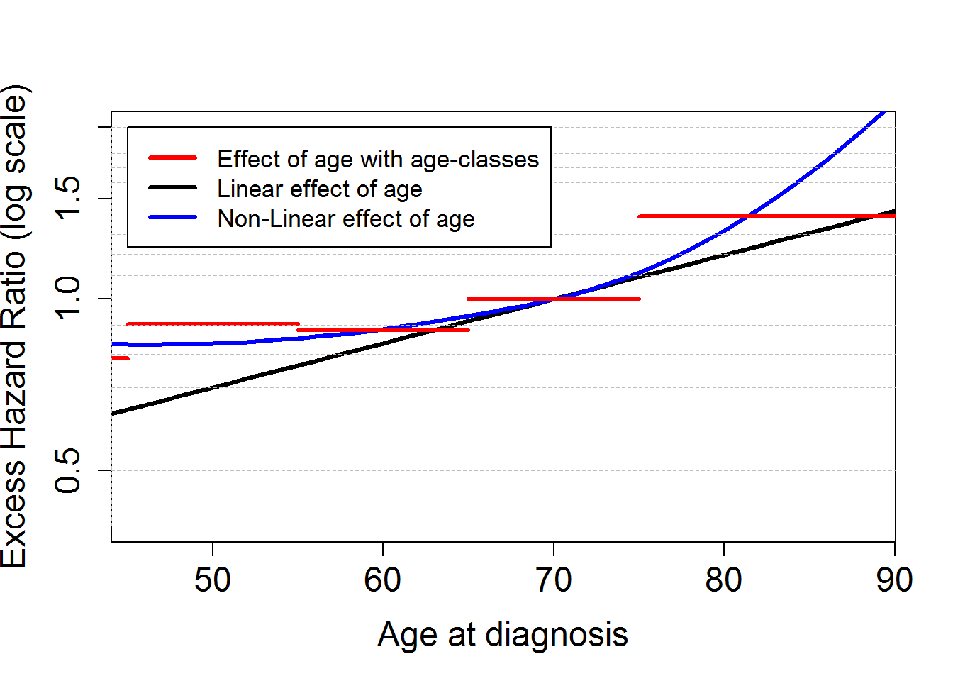
Fourth Model: Age analysed assuming a Non-linear and a Time-dependent effect
We fit a model M4bs assuming a cubic B-spline function for the (log of the ) baseline excess hazard (arguments base="exp.bs" and degree=3), with one knot located at 1 year (argument knots to specify the location of the knot(s)). The model M4bs assumes proportional (i.e. constant over time) effects of the covariables dep and stage, and a non-linear and time-dependent effect of continuous age. The excess mortality hazard fitted is of the form \[ \lambda_E(t; x) = \lambda_0(t)\exp \big(\sum_{i=2}^4 \alpha_i stage_i + \sum_{i=2}^5 \beta_i dep_i + \beta_a(t) agec + f(agec) \big)\]. To fit this very complicated model, it’s useful to speed-up the optimisation process and to ensure reaching convergence to start by fitting a model for the overall hazard, and to use the parameters estimated from this model as initial values for the excess hazard regression model.
Estimation
M4bsoverall <- mexhaz(Surv(timey, dead)~Idep2+Idep3+Idep4+Idep5+IstageB+IstageC+IstageD+
                        agediagc+ agediagc2+ agediagc2plus+ nph(agediagc),
                      data=temp, base="exp.bs", degree=3, knots=c(1), verbose=0)
## iteration = 0
## Step:
## [1] 0 0 0 0 0 0 0 0 0 0 0 0 0 0 0 0 0 0 0
## Parameter:
## [1] -1 -1 -1 -1 -1 0 0 0 0 0 0 0 0 0 0 0 0 0 0
## Function Value
## [1] 29263.43
## Gradient:
## [1] -1454.52510 -1009.66127 44.08982 412.48073 292.48885
## [6] -134.46506 -284.92816 -483.78169 -523.70191 1277.60311
## [11] -1193.44837 -2196.44311 -34454.89916 -229928.59448 -374049.44891
## [16] -8855.78410 -6096.80895 -5680.60689 -2912.08740
##
## iteration = 282
## Parameter:
## [1] -1.5007237982 -1.4781714121 -0.8149265313 -2.4986976124 -1.7847442126
## [6] 0.0253381932 0.0951811483 0.1663045151 0.2726671179 0.3545031956
## [11] 1.0322656441 2.2815964098 0.0629500273 0.0006338815 0.0002258313
## [16] -0.0455737374 -0.0452616366 0.0131342679 0.0075273268
## Function Value
## [1] 24965.59
## Gradient:
## [1] 2.666564e-05 -2.461135e-06 -3.637979e-06 1.019165e-05 6.115126e-06
## [6] -4.729372e-05 -6.912160e-05 1.200533e-04 2.910383e-05 -2.546585e-05
## [11] 2.819413e-05 1.913386e-05 1.946319e-03 -8.618372e-03 2.314846e-02
## [16] 4.947651e-04 1.127773e-04 4.401954e-04 3.310561e-04
##
## Gradient relatif proche de zéro.
## L'itération courante est probablement la solution.
##
## Computation of the Hessian
##
## Data
## Name N.Obs.Tot N.Obs N.Events N.Clust
## temp 17867 17867 10972 1
##
## Details
## Iter Eval Base Nb.Leg Nb.Aghq Optim Method Code LogLik Total.Time
## 282 4423 exp.bs 20 10 nlm --- 1 -24965.59 267.34initial <- round(M4bsoverall$coeff,2)
M4bs <- mexhaz(Surv(timey, dead)~Idep2+Idep3+Idep4+Idep5+IstageB+IstageC+IstageD+
agediagc+ agediagc2+ agediagc2plus+ nph(agediagc),
data=temp, base="exp.bs", degree=3, knots=c(1), verbose=0, expected="rate", init=initial)## iteration = 0
## Step:
## [1] 0 0 0 0 0 0 0 0 0 0 0 0 0 0 0 0 0 0 0
## Parameter:
## [1] -1.50 -1.48 -0.81 -2.50 -1.78 0.03 0.10 0.17 0.27 0.35 1.03
## [12] 2.28 0.06 0.00 0.00 -0.05 -0.05 0.01 0.01
## Function Value
## [1] 22169.74
## Gradient:
## [1] 1309.1132 432.1932 431.9112 343.4226 153.0077
## [6] 269.6434 279.1382 301.1285 252.0926 788.7615
## [11] 413.9940 -117.1938 8363.2069 -10558.9898 69174.5661
## [16] 3533.2166 2897.2204 1989.5366 811.7438
##
## iteration = 256
## Parameter:
## [1] -2.191920461 -1.692536222 -0.727363895 -3.733211392 -3.060946755
## [6] -0.013513911 0.066841749 0.116197303 0.218633102 0.829855130
## [11] 1.810852104 3.142993552 0.064570026 0.000177123 0.000328597
## [16] -0.066693262 -0.056157804 -0.060386972 -0.065451875
## Function Value
## [1] 21689.32
## Gradient:
## [1] -2.224028e-04 -7.522986e-05 1.455192e-05 -4.775003e-05 -1.212285e-04
## [6] -3.201421e-04 -7.639755e-05 -1.273293e-04 3.274181e-04 -9.094947e-05
## [11] -8.839544e-05 -1.261662e-04 -1.342414e-03 -7.305061e-03 -1.066655e-02
## [16] -1.164153e-04 -7.057679e-04 -2.837623e-04 -2.437446e-04
##
## Gradient relatif proche de zéro.
## L'itération courante est probablement la solution.
##
## Computation of the Hessian
##
## Data
## Name N.Obs.Tot N.Obs N.Events N.Clust
## temp 17867 17867 10972 1
##
## Details
## Iter Eval Base Nb.Leg Nb.Aghq Optim Method Code LogLik Total.Time
## 256 3778 exp.bs 20 10 nlm --- 1 -21689.32 220.77summary(M4bs)## Call:
## mexhaz(formula = Surv(timey, dead) ~ Idep2 + Idep3 + Idep4 +
## Idep5 + IstageB + IstageC + IstageD + agediagc + agediagc2 +
## agediagc2plus + nph(agediagc), data = temp, expected = "rate",
## base = "exp.bs", degree = 3, knots = c(1), init = initial,
## verbose = 0)
##
## Coefficients:
## Estimate StdErr t.value p.value
## Intercept -2.19192046 0.10979383 -19.9640 < 2.2e-16 ***
## BS3.1 -1.69253622 0.06564902 -25.7816 < 2.2e-16 ***
## BS3.2 -0.72736390 0.13495625 -5.3896 7.150e-08 ***
## BS3.3 -3.73321139 0.28372563 -13.1578 < 2.2e-16 ***
## BS3.4 -3.06094675 0.39966416 -7.6588 1.972e-14 ***
## Idep2 -0.01351391 0.03970917 -0.3403 0.733618
## Idep3 0.06684175 0.03976988 1.6807 0.092836 .
## Idep4 0.11619730 0.03944915 2.9455 0.003229 **
## Idep5 0.21863310 0.04024356 5.4327 5.622e-08 ***
## IstageB 0.82985513 0.10508461 7.8970 3.021e-15 ***
## IstageC 1.81085210 0.10254793 17.6586 < 2.2e-16 ***
## IstageD 3.14299355 0.10307628 30.4919 < 2.2e-16 ***
## agediagc 0.06457003 0.00434106 14.8742 < 2.2e-16 ***
## agediagc2 0.00017712 0.00010463 1.6929 0.090489 .
## agediagc2plus 0.00032860 0.00030008 1.0950 0.273525
## agediagc*BS3.1 -0.06669326 0.00598991 -11.1343 < 2.2e-16 ***
## agediagc*BS3.2 -0.05615780 0.01137211 -4.9382 7.956e-07 ***
## agediagc*BS3.3 -0.06038697 0.02266408 -2.6644 0.007719 **
## agediagc*BS3.4 -0.06545187 0.02916930 -2.2439 0.024854 *
## ---
## Signif. codes: 0 '***' 0.001 '**' 0.01 '*' 0.05 '.' 0.1 ' ' 1
##
## Hazard ratios (for proportional effect variables):
## Coef HR CI.lower CI.upper
## Idep2 -0.0135 0.9866 0.9127 1.0664
## Idep3 0.0668 1.0691 0.9890 1.1558
## Idep4 0.1162 1.1232 1.0396 1.2135
## Idep5 0.2186 1.2444 1.1500 1.3465
## IstageB 0.8299 2.2930 1.8662 2.8174
## IstageC 1.8109 6.1157 5.0021 7.4772
## IstageD 3.1430 23.1731 18.9339 28.3615
## agediagc 0.0646 1.0667 1.0577 1.0758
## agediagc2 0.0002 1.0002 1.0000 1.0004
## agediagc2plus 0.0003 1.0003 0.9997 1.0009
##
## log-likelihood: -21689.3213 (for 19 degree(s) of freedom)
##
## number of observations: 17867, number of events: 10972Prediction
myagediag <- 50
myagediagc <- myagediag-70
myagediagc2 <- myagediagc^2
myagediagc2plus <- (myagediagc-0)^2*(myagediagc>0)
predM4bsage50 <- predict.mexhaz(M4bs, time.pts = mytime,
                                data.val = data.frame(Idep2=0, Idep3=0, Idep4=0, Idep5=0,
                                                      IstageB=0, IstageC=0, IstageD=0,
                                                      agediagc=myagediagc, agediagc2=myagediagc2, agediagc2plus=myagediagc2plus))
myagediag <- 60
myagediagc <- myagediag-70
myagediagc2 <- myagediagc^2
myagediagc2plus <- (myagediagc-0)^2*(myagediagc>0)
predM4bsage60 <- predict.mexhaz(M4bs, time.pts = mytime,
                                data.val = data.frame(Idep2=0, Idep3=0, Idep4=0, Idep5=0,
                                                      IstageB=0, IstageC=0, IstageD=0,
                                                      agediagc=myagediagc, agediagc2=myagediagc2, agediagc2plus=myagediagc2plus))
myagediag <- 70
myagediagc <- myagediag-70
myagediagc2 <- myagediagc^2
myagediagc2plus <- (myagediagc-0)^2*(myagediagc>0)
predM4bsage70 <- predict.mexhaz(M4bs, time.pts = mytime,
                                data.val = data.frame(Idep2=0, Idep3=0, Idep4=0, Idep5=0,
                                                      IstageB=0, IstageC=0, IstageD=0,
                                                      agediagc=myagediagc, agediagc2=myagediagc2, agediagc2plus=myagediagc2plus))

myagediag <- 80
myagediagc <- myagediag-70
myagediagc2 <- myagediagc^2
myagediagc2plus <- (myagediagc-0)^2*(myagediagc>0)
predM4bsage80 <- predict.mexhaz(M4bs, time.pts = mytime,
                                data.val = data.frame(Idep2=0, Idep3=0, Idep4=0, Idep5=0,
                                                      IstageB=0, IstageC=0, IstageD=0,
                                                      agediagc=myagediagc, agediagc2=myagediagc2, agediagc2plus=myagediagc2plus))
par(mar=c(5,4,4,2)+0.1)
plot(0,1, xlim=c(0,5),ylim=c(0,0.15), type="n",
     xlab="Time since diagnosis",ylab="Excess Hazard",cex.lab=1.5, cex.axis=1.5, cex=1.5)
points(predM4bsage50, which="hazard", lwd=3, col="green", conf.int = F)
points(predM4bsage60, which="hazard", lwd=3, col="orange",lty.pe=4, conf.int = F)
points(predM4bsage70, which="hazard", lwd=3, col="blue",lty.pe=2, conf.int = F)
points(predM4bsage80, which="hazard", lwd=3, col="red",lty.pe=6, conf.int = F)
axis(2,at=seq(0,0.25,by=0.05), tck=1,lty=8, lwd=0.1, labels=F, col="grey")
title("Estimates of the excess hazard for different ages", cex.main=1.5)
mtext("Men, Stage A, Deprivation level 1", cex=1.2)
legend(1,0.15,c("50 years old", "60 years old", "70 years old", "80 years old"),
       col=c("green", "orange", "blue", "red"), lty=c(1,4,2,6), lwd=3,cex=1.5, bg="white")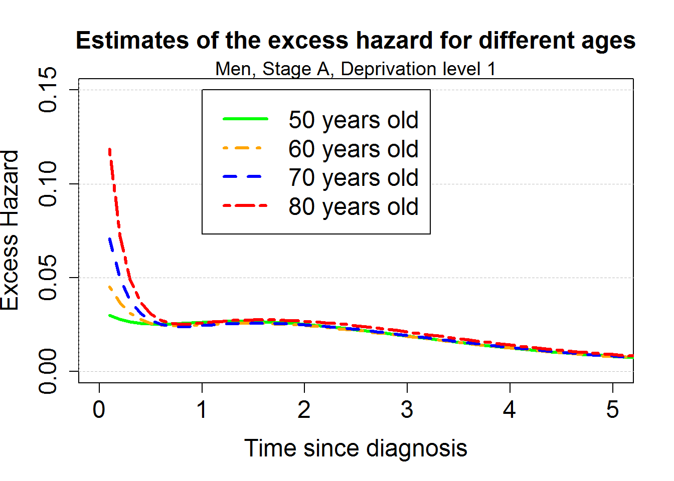
excratefixnlinnphage <- data.frame(Thetime=mytime)
rangeage <- seq(35,90,by=1)

for (agestudy in rangeage){
  myagediag <- agestudy
  myagediagc <- myagediag-70
  myagediagc2 <- myagediagc^2
  myagediagc2plus <- (myagediagc-0)^2*(myagediagc>0)
  predage <- predict.mexhaz(M4bs, time.pts = mytime,
                              data.val = data.frame(Idep2=0, Idep3=0, Idep4=0, Idep5=0,
                                                    IstageB=0, IstageC=0, IstageD=0,
                                                  agediagc=myagediagc, agediagc2=myagediagc2, agediagc2plus=myagediagc2plus))
  excratefixnlinnphage[,paste0("age",agestudy)] <- predage$results$hazard
  }


par(mar=c(5,4,4,2)+0.1)
plot(0, 0 , type="n",
     xlim=c(min(rangeage),max(rangeage)),ylim=c(0,2),
     xlab="Age at diagnosis",ylab="Excess hazard ratio",cex.lab=1.5, cex.axis=1.5, cex=1.5
)
lines(rangeage, excratefixnlinnphage[excratefixnlinnphage$Thetime=="0.3",][-1]/excratefixnlinnphage[excratefixnlinnphage$Thetime=="0.3",c("age70")], lwd=3, col="red")
lines(rangeage, excratefixnlinnphage[excratefixnlinnphage$Thetime=="5",][-1]/excratefixnlinnphage[excratefixnlinnphage$Thetime=="5",c("age70")], lwd=3, col="blue", lty=4)
axis(2,at=seq(0,2,by=0.2), tck=1,lty=8, lwd=0.1, labels=F, col="grey")
axis(2, label=F, at=1, tck=1,lty=1, lwd=0.2)
axis(1, label=F, at=70, tck=1,lty=8, lwd=0.2)
title("Estimated non-linear effect of age at different times", cex.main=1.5)
mtext("Men, Stage A, Deprivation level 1", cex=1.2)
legend(36,2,c("Non-Linear effect of age at 4 month", "Non-Linear effect of age at 5 years"),
       col=c("red", "blue"), lty=c(1,4), lwd=3, cex=1.3, bg="white")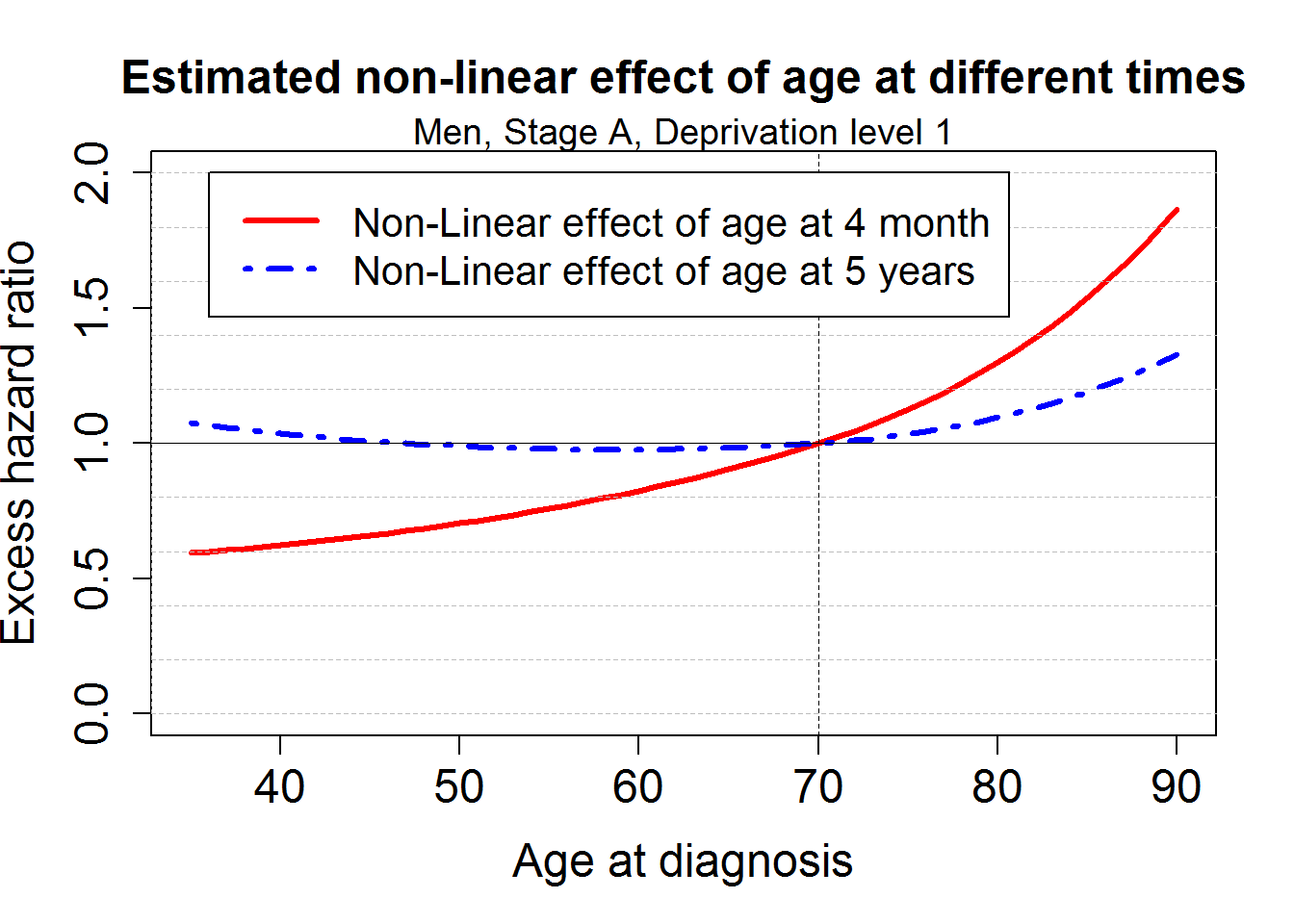
par(mar=c(5,4,4,2)+0.1)
z <- excratefixnlinnphage[,-1]
persp(x=rangeage, y=mytime, z = t(as.matrix(z)), xlab="Age at diagnosis",ylab="Time since diagnosis", zlab="Excess hazard",
      theta = 120, phi = 20, expand = 0.5, col = "lightblue",
      xlim=c(min(rangeage),max(rangeage)), ylim=c(min(mytime),max(mytime)), shade = 0.75, ticktype = "detailed" )
title("Excess hazard according to \n time since diagnosis and age at diagnosis", cex.main=1.2)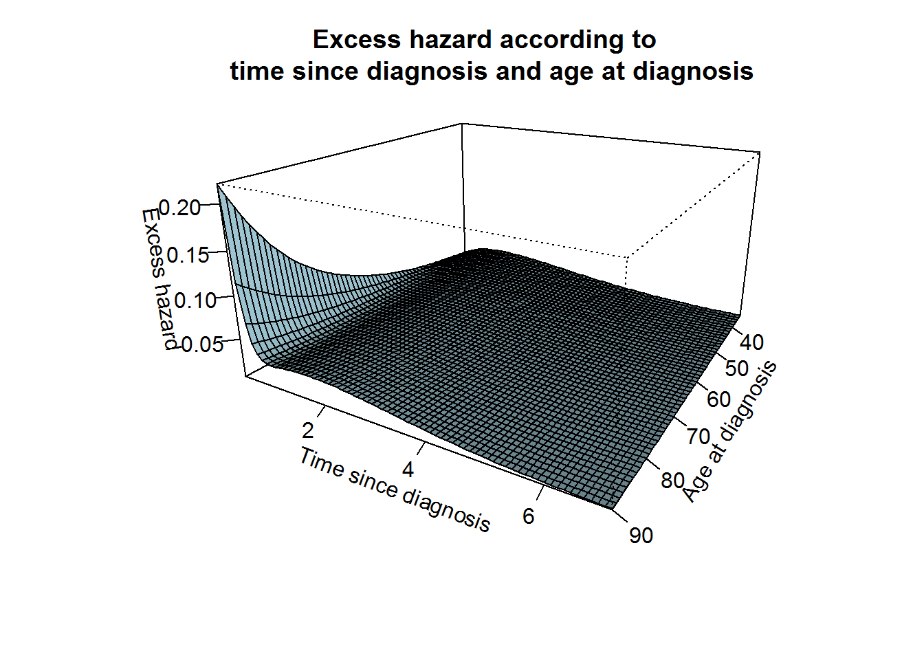
Model comparison
After fitting the three models with different complexity of the association between age at diagnosis and the excess hazard regression model, the natural question is to assess which of those 3 models provide the better fit. The Akaike Information Criterion calculated below shows that the fourth model (non-linear and time-dependent effect of age) provides the better fit.
Akaike Information Criterion
#LOG-LIKELIHOOD
M2bs$loglik
## [1] -21880.73M3bs$loglik## [1] -21840.06M4bs$loglik## [1] -21689.32# AKAIKE INFORMATION CRITERIA
-2 * M2bs$loglik + 2 * M2bs$n.par## [1] 43787.46-2 * M3bs$loglik + 2 * M3bs$n.par## [1] 43710.12-2 * M4bs$loglik + 2 * M4bs$n.par## [1] 43416.64Comparison of the excess mortality hazard and the net survival estimated from the 3 different models for a 80 years old patient
We can compare the estimated values of the excess hazard and the corresponding net survival obtained from the 3 different models for specific age.
myagediag <- 80
myagediagc <- myagediag-70
myagediagc2 <- myagediagc^2
myagediagc2plus <- (myagediagc-0)^2*(myagediagc>0)

predagelin <- predict.mexhaz(M2bs, time.pts = mytime,
                           data.val = data.frame(Idep2=0, Idep3=0, Idep4=0, Idep5=0,
                                                 IstageB=0, IstageC=0, IstageD=0,
                                                 agediagc=myagediagc))
predageNlin <- predict.mexhaz(M3bs, time.pts = mytime,
                               data.val = data.frame(Idep2=0, Idep3=0, Idep4=0, Idep5=0,
                                                     IstageB=0, IstageC=0, IstageD=0,
                                                     agediagc=myagediagc, agediagc2=myagediagc2, agediagc2plus=myagediagc2plus))
predageNlinTD <- predict.mexhaz(M4bs, time.pts = mytime,
                               data.val = data.frame(Idep2=0, Idep3=0, Idep4=0, Idep5=0,
                                                     IstageB=0, IstageC=0, IstageD=0,
                                                     agediagc=myagediagc, agediagc2=myagediagc2, agediagc2plus=myagediagc2plus))

par(mar=c(5,4,4,2)+0.1)
plot(predagelin, which="hazard", conf.int=F, lwd=2, lty.pe=2)
points(predageNlin, which="hazard", col="blue", conf.int=F, lwd=2, lty.pe=4)
points(predageNlinTD, which="hazard", col="green", conf.int=F, lwd=2)
axis(2,at=seq(0,1,by=0.02), tck=1,lty=8, lwd=0.1, labels=F, col="grey")
title("Excess mortality hazard estimated from the different models", cex.main=1.2)
mtext("80 years old -  Men, Stage A, Deprivation level 1", cex=1.2)
legend(0.5,0.08,c("Linear effect of age", "Non-Linear effect of age", "Non-linear & time-dependent effect of age"),
       col=c("black", "blue", "green"), lty=c(2,4,1), lwd=3,cex=1.2, bg="white")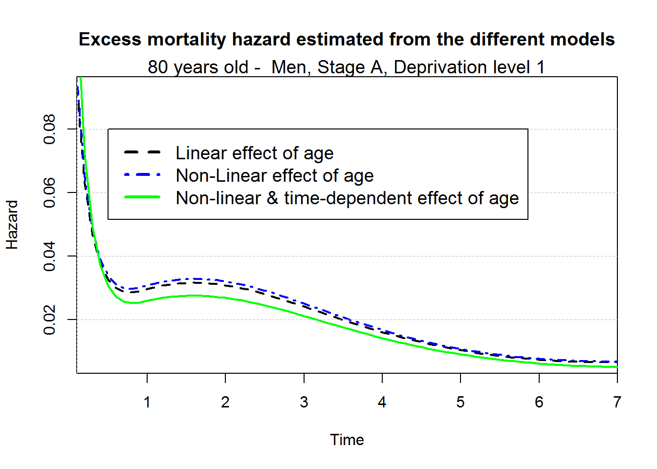
par(mar=c(5,4,4,2)+0.1)
plot(0, 0, type="n", xlim=c(0,5),ylim=c(0.80,1),
     xlab="Time since diagnosis",ylab="Net Survival",cex.lab=1.5, cex.axis=1.5, cex=1.5)
points(predagelin, which="surv", conf.int=F, lwd=2, lty.pe=2)
points(predageNlin, which="surv", col="blue", conf.int=F, lwd=2, lty.pe=4)
points(predageNlinTD, which="surv", col="green", conf.int=F, lwd=2)

axis(2,at=seq(0,1,by=0.05), tck=1,lty=8, lwd=0.1, labels=F, col="grey")
title("Net survival estimated using the different models", cex.main=1.5)
mtext("80 years old -  Men, Stage A, Deprivation level 1", cex=1.2)
legend(0,0.87,c("Linear effect of age", "Non-Linear effect of age", "Non-linear & time-dependent effect of age"),
       col=c("black", "blue", "green"), lty=c(2,4,1), lwd=3,cex=1.2, bg="white")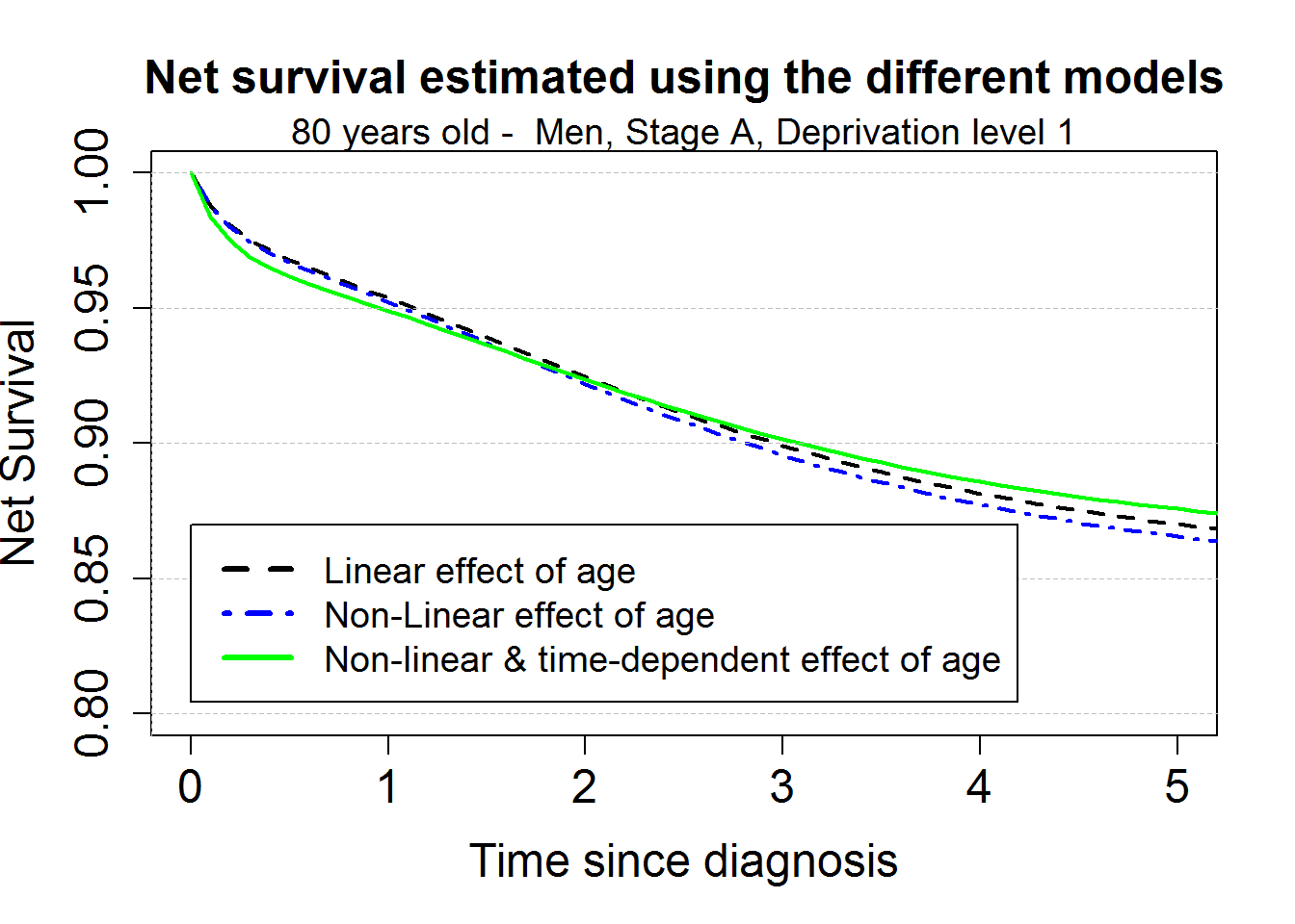
Comparison of the excess mortality hazard and the net survival estimated from the 3 different models for a 55 years old patient
myagediag <- 55
myagediagc <- myagediag-70
myagediagc2 <- myagediagc^2
myagediagc2plus <- (myagediagc-0)^2*(myagediagc>0)

predagelin <- predict.mexhaz(M2bs, time.pts = mytime,
                             data.val = data.frame(Idep2=0, Idep3=0, Idep4=0, Idep5=0,
                                                   IstageB=0, IstageC=0, IstageD=0,
                                                   agediagc=myagediagc))
predageNlin <- predict.mexhaz(M3bs, time.pts = mytime,
                              data.val = data.frame(Idep2=0, Idep3=0, Idep4=0, Idep5=0,
                                                    IstageB=0, IstageC=0, IstageD=0,
                                                    agediagc=myagediagc, agediagc2=myagediagc2, agediagc2plus=myagediagc2plus))
predageNlinTD <- predict.mexhaz(M4bs, time.pts = mytime,
                                data.val = data.frame(Idep2=0, Idep3=0, Idep4=0, Idep5=0,
                                                      IstageB=0, IstageC=0, IstageD=0,
                                                      agediagc=myagediagc, agediagc2=myagediagc2, agediagc2plus=myagediagc2plus))

par(mar=c(5,4,4,2)+0.1)
plot(predagelin, which="hazard", conf.int=F, lwd=2, lty.pe=2)
points(predageNlin, which="hazard", col="blue", conf.int=F, lwd=2, lty.pe=4)
points(predageNlinTD, which="hazard", col="green", conf.int=F, lwd=2)
axis(2,at=seq(0,1,by=0.02), tck=1,lty=8, lwd=0.1, labels=F, col="grey")
title("Excess mortality hazard estimated from the different models", cex.main=1.2)
mtext("55 years -  Men, Stage A, Deprivation level 1", cex=1.2)
legend(0.5,0.06,c("Linear effect of age", "Non-Linear effect of age", "Non-linear & time-dependent effect of age"),
       col=c("black", "blue", "green"), lty=c(2,4,1), lwd=3,cex=1.2, bg="white")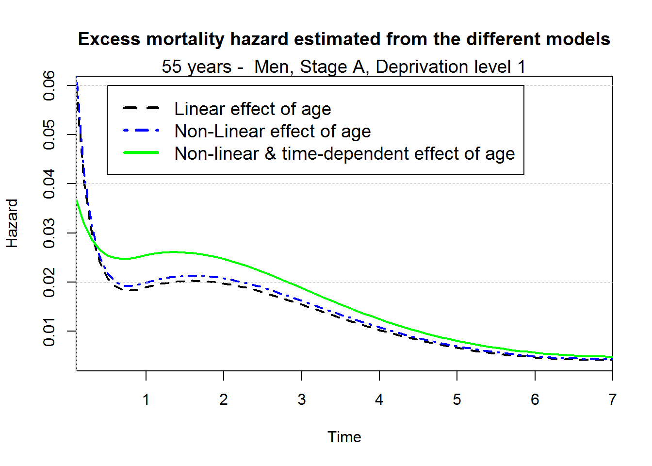
par(mar=c(5,4,4,2)+0.1)
plot(0, 0, type="n", xlim=c(0,5),ylim=c(0.80,1),
     xlab="Time since diagnosis",ylab="Net Survival",cex.lab=1.5, cex.axis=1.5, cex=1.5)
points(predagelin, which="surv", conf.int=F, lwd=2, lty.pe=2)
points(predageNlin, which="surv", col="blue", conf.int=F, lwd=2, lty.pe=4)
points(predageNlinTD, which="surv", col="green", conf.int=F, lwd=2)

axis(2,at=seq(0,1,by=0.05), tck=1,lty=8, lwd=0.1, labels=F, col="grey")
title("Net survival estimated from the different models", cex.main=1.5)
mtext("55 years -  Men, Stage A, Deprivation level 1", cex=1.2)
legend(0,0.88,c("Linear effect of age", "Non-Linear effect of age", "Non-linear & time-dependent effect of age"),
       col=c("black", "blue", "green"), lty=c(2,4,1), lwd=3,cex=1.2, bg="white")